Alpha diversity

In the previous section, I explored the bacteria that were present in the samples and in the positive and negative sequencing controls. Now I move on to alpha diversity, which is a measure of the diversity within samples; essentially we are asking, “how complex are these communities?”

I chose to calculate the diversity within samples using two different metrics; one phylogenetic metric (i.e. takes into account the relatedness of the bacteria) and one non-phylogenetic metric (doesn’t take this into account). I then compared the alpha diversity value between groups of samples.

I began with the OTU table that contains only samples above 1499 reads. However, we need to account for variations in sequencing depth so I cannot use the raw counts here. For example, if we compare sample A with 100,000 reads to sample B with 10,000 reads, the diversity in sample A will probably be greater just because we have a greater sampling depth. One way to account for this (and which is commonly used) is to rarefy the samples: choosing a threshold to which you will subsample the reads at random to end up with the same number of reads per sample. This may work, but it reduces statistical power by chucking out usable data and in the case of our study, this was a lot of data.

So I have instead employed cumulative-sum-scaling (CSS) normalisation, which can be found in the bioConductor package metagenomeSeq. I use this package further in the differential abundance analysis, but for now I am just using it to normalise the OTU table.

Calculating alpha diversity in QIIME

Firstly, creating the normalised version of the OTU table with metagenomeSeq:

library(metagenomeSeq)
# Create a metagenomeSeq object for the raw OTU table

# OTU counts
table.alpha <- loadMeta("data/final_otu_table_samples.txt", sep = "\t")

# OTU taxonomy: taken from OTU table and separated by tabs
taxa <- read.delim("data/taxonomy_raw.txt", stringsAsFactors = FALSE, sep = "\t")
OTUdata <- AnnotatedDataFrame(taxa)
row.names(OTUdata) <- taxa$taxa
OTUdata

## An object of class 'AnnotatedDataFrame'
##   rowNames: OTU5 OTU2 ... OTU52 (123 total)
##   varLabels: taxa Kingdom ... X (8 total)
##   varMetadata: labelDescription

# Full object
alphadata <- newMRexperiment(table.alpha$counts, featureData = OTUdata)
alphadata

## MRexperiment (storageMode: environment)
## assayData: 123 features, 481 samples 
##   element names: counts 
## protocolData: none
## phenoData: none
## featureData
##   featureNames: OTU5 OTU2 ... OTU52 (123 total)
##   fvarLabels: taxa Kingdom ... X (8 total)
##   fvarMetadata: labelDescription
## experimentData: use 'experimentData(object)'
## Annotation:

Now that the data is in metagenomeSeq’s format, I normalise the counts:

p <- cumNormStatFast(alphadata)

## Default value being used.

alphadata <- cumNorm(alphadata, p = p)

# Export normalised and logged matrix for use in alpha diversity
alphanorm <- MRcounts(alphadata, norm = TRUE, log = TRUE)
#write.table(alphanorm, "alphadata_normalised.txt", sep = "\t")

Now I move to QIIME with this table.

# First convert back to biom format (the table was JSON format before)
biom convert -i alphadata_normalised.txt -o alphadata_normalised.biom --table-type="OTU table" --to-json

# Run alpha diversity on this table
alpha_diversity.py -i alphadata_normalised.biom -m PD_whole_tree,simpson_reciprocal -o
alpha_div_normalised.txt -t ../rep_set.tre

The above script uses the phylogenetic tree that I made when pre-processing the data; the PD_whole_tree method (Faith’s Phylogenetic Diversity) requires this. The other metric is inverse (or reciprocal) Simpson.

Plotting alpha diversity in R

I bring the resulting file back into R to plot the alpha diversity.

alphadiv.normal <- read.table("data/alpha_div_normalised.txt", sep = "\t", header = T)
# Split into PD and Simpson metrics
PD.normal <- alphadiv.normal[,1:2]
simp.normal <- alphadiv.normal[,-2]
names(PD.normal) <- c("SampleID", "PD_whole_tree")
names(simp.normal) <- c("SampleID", "simpson_reciprocal")

Testing for differences between groups

I have the alpha diversity value for each sample, but I am interested in grouping them by sample type and comparing the alpha diversity of these groups.

I added the sample type to the data using my initial basic version of the mapping file I had in QIIME:

# Add metadata
library(qiimer)
map <- read_qiime_mapping_file("data/mapfile_Runs1234.txt")
PD.data <- merge(map, PD.normal, by = "SampleID")
PD.data$sample_type <- droplevels(PD.data$sample_type)
Simp.data <- merge(map, simp.normal, by = "SampleID")
Simp.data$sample_type <- droplevels(Simp.data$sample_type)

Now I tested for differences between groups (defined by sample type) for both metrics.

1. Case and control NPS

# Subset to the NPS samples for PD
case.controlPD <- PD.data[grep("control|NPS", PD.data$sample_type),]
case.controlPD$sample_type <- droplevels(case.controlPD$sample_type)

# Subset to the NPS samples for Simpson
case.controlSimp <- Simp.data[grep("control|NPS", Simp.data$sample_type),]
case.controlSimp$sample_type <- droplevels(case.controlSimp$sample_type)

# Test for difference in PD value (non-parametric)
wilcox.test(PD_whole_tree ~ sample_type, data = case.controlPD)

## 
##  Wilcoxon rank sum test with continuity correction
## 
## data:  PD_whole_tree by sample_type
## W = 2583, p-value = 1.142e-06
## alternative hypothesis: true location shift is not equal to 0

# Test for difference in Simp value (non-parametric)
wilcox.test(simpson_reciprocal ~ sample_type, data = case.controlSimp)

## 
##  Wilcoxon rank sum test with continuity correction
## 
## data:  simpson_reciprocal by sample_type
## W = 2278.5, p-value = 1.316e-08
## alternative hypothesis: true location shift is not equal to 0

2. Middle ear fluid and middle ear rinse

For this comparison, the samples are no longer independent because they come from the same child. In this case, I needed to do a paired test so as to not violate the independent samples assumption.

In my differential abundance analysis (explained in detail in a later section) I selected at random a set of fluid and rinse pairs from the same ear of the same child, with each child contributing only one pair.

# Subset data to fluids and rinses only
fluid.rinsePD <- PD.data[grep("fluid|rinse", PD.data$sample_type),]
fluid.rinsePD$sample_type <- droplevels(fluid.rinsePD$sample_type)

fluid.rinseSimp <- Simp.data[grep("fluid|rinse", Simp.data$sample_type),]
fluid.rinseSimp$sample_type <- droplevels(fluid.rinseSimp$sample_type)

# Read in the list of pairs that I previously chose
FRsamples <- read.table("data/FRsamples.txt", header = T, sep = "\t")
names(FRsamples) <- c("SampleID", "ID", "type")

# Subset data to these chosen pairs
fluid.rinsePD <- merge(fluid.rinsePD, FRsamples, by = "SampleID")
fluid.rinseSimp <- merge(fluid.rinseSimp, FRsamples, by = "SampleID")

# Split into fluids and rinses
fluidPD <- fluid.rinsePD[grep("fluid",fluid.rinsePD$sample_type),]
fluidPD$sample_type <- droplevels(fluidPD$sample_type)         
rinsePD <- fluid.rinsePD[grep("rinse",fluid.rinsePD$sample_type),]
rinsePD$sample_type <- droplevels(rinsePD$sample_type)         

fluidSimp <- fluid.rinseSimp[grep("fluid",fluid.rinseSimp$sample_type),]
fluidSimp$sample_type <- droplevels(fluidSimp$sample_type)         
rinseSimp <- fluid.rinseSimp[grep("rinse",fluid.rinseSimp$sample_type),]
rinseSimp$sample_type <- droplevels(rinseSimp$sample_type)     

# Check that the fluids and rinses are in the same order (so the test knows which are paired)
test1 <- ifelse(fluidPD$ID == rinsePD$ID, T, F)
test2 <- ifelse(fluidSimp$ID == rinseSimp$ID, T, F)

# Test for differences between groups using non-parametric paired test
wilcox.test(fluidPD$PD_whole_tree, rinsePD$PD_whole_tree, paired = T)

## 
##  Wilcoxon signed rank test with continuity correction
## 
## data:  fluidPD$PD_whole_tree and rinsePD$PD_whole_tree
## V = 357, p-value = 0.006873
## alternative hypothesis: true location shift is not equal to 0

wilcox.test(fluidSimp$simpson_reciprocal, rinseSimp$simpson_reciprocal, paired = T)

## 
##  Wilcoxon signed rank test with continuity correction
## 
## data:  fluidSimp$simpson_reciprocal and rinseSimp$simpson_reciprocal
## V = 391, p-value = 0.01756
## alternative hypothesis: true location shift is not equal to 0

3. Middle ear fluid and nasopharynx

Again, these samples are from within the same children and I am using pairs which I previously selected.

# Subset data to fluids and NPS only (not controls)
fluid.npsPD <- PD.data[grep("fluid|NPS", PD.data$sample_type),]
fluid.npsPD$sample_type <- droplevels(fluid.npsPD$sample_type)

fluid.npsSimp <- Simp.data[grep("fluid|NPS", Simp.data$sample_type),]
fluid.npsSimp$sample_type <- droplevels(fluid.npsSimp$sample_type)

# Read in the previously chosen pairs
FNPSsamples <- read.table("data/FNPSsamples.txt", header = T, sep = "\t")
names(FNPSsamples) <- c("SampleID", "ID", "type")

# Subset data to these chosen samples
fluid.npsPD <- merge(fluid.npsPD, FNPSsamples, by = "SampleID")
fluid.npsSimp <- merge(fluid.npsSimp, FNPSsamples, by = "SampleID")

# Split into fluids and NPS (this set of fluids is different to the set used in the fluid/rinse comparison)
fluidPD2 <- fluid.npsPD[grep("fluid",fluid.npsPD$sample_type),]
fluidPD2$sample_type <- droplevels(fluidPD2$sample_type)         
npsPD <- fluid.npsPD[grep("NPS",fluid.npsPD$sample_type),]
npsPD$sample_type <- droplevels(npsPD$sample_type)         

fluidSimp2 <- fluid.npsSimp[grep("fluid",fluid.npsSimp$sample_type),]
fluidSimp2$sample_type <- droplevels(fluidSimp2$sample_type)         
npsSimp <- fluid.npsSimp[grep("NPS",fluid.npsSimp$sample_type),]
npsSimp$sample_type <- droplevels(npsSimp$sample_type)  

# Check they are in the right order
test3 <- ifelse(fluidPD2$ID == npsPD$ID, T, F)
test4 <- ifelse(fluidSimp2$ID == npsSimp$ID, T, F)

# Test for differences between groups with non-parametric paired test
wilcox.test(fluidPD2$PD_whole_tree, npsPD$PD_whole_tree, paired = T)

## 
##  Wilcoxon signed rank test with continuity correction
## 
## data:  fluidPD2$PD_whole_tree and npsPD$PD_whole_tree
## V = 125, p-value = 6.786e-12
## alternative hypothesis: true location shift is not equal to 0

wilcox.test(fluidSimp2$simpson_reciprocal, npsSimp$simpson_reciprocal, paired = T)

## 
##  Wilcoxon signed rank test with continuity correction
## 
## data:  fluidSimp2$simpson_reciprocal and npsSimp$simpson_reciprocal
## V = 116, p-value = 4.86e-12
## alternative hypothesis: true location shift is not equal to 0

Creating one large plot

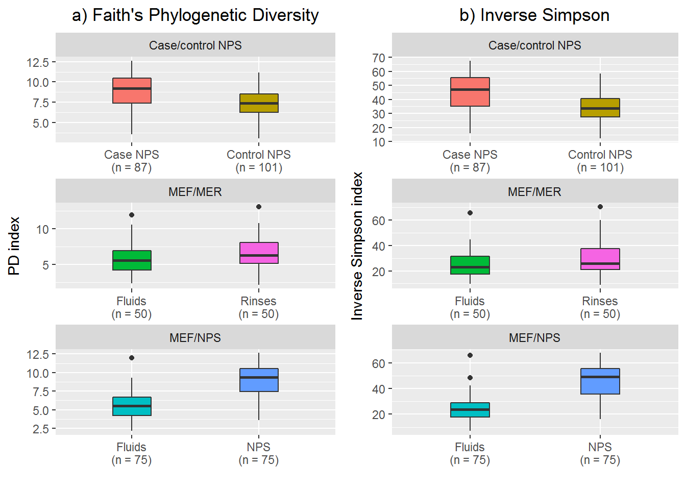
Now I have determined the p-values for the differences between groups, I wanted to present the data as boxplots.

Note that I could not manage to put the p-values on the plot (not six different ones at least) so for the final figure in the paper I added the p-values using Inkscape.

I used ggplot2 to create two faceted plots. Each plot contained three facets (the three comparisons) with one plot for PD, one for inverse Simp. I then arranged these plots next to each other.

First, I had to do some data wrangling.

Cases and controls:

# Remove unnecessary data that came from mapping file
case.controlPD <- data.frame(case.controlPD$SampleID, case.controlPD$sample_type, case.controlPD$PD_whole_tree)
names(case.controlPD) <- c("Sample_ID", "sample_type", "PD_whole_tree")

case.controlSimp <- data.frame(case.controlSimp$SampleID, case.controlSimp$sample_type, case.controlSimp$simpson_reciprocal)
names(case.controlSimp) <- c("Sample_ID", "sample_type", "simpson_reciprocal")

# Specify case group (different to NPS in fluid/NPS comparison)
case.controlPD$sample_type <- gsub("NPS", "case", case.controlPD$sample_type)
case.controlSimp$sample_type <- gsub("NPS", "case", case.controlSimp$sample_type)

# Combine the data for facet 1
data1 <- merge(case.controlPD, case.controlSimp)

Fluids and rinses:

# Remove unnecessary data
fluidPD <- data.frame(fluidPD$SampleID, fluidPD$sample_type, fluidPD$PD_whole_tree)
rinsePD <- data.frame(rinsePD$SampleID, rinsePD$sample_type, rinsePD$PD_whole_tree)
names(fluidPD) <- c("Sample_ID", "sample_type", "PD_whole_tree")
names(rinsePD) <- c("Sample_ID", "sample_type", "PD_whole_tree")

fluidSimp <- data.frame(fluidSimp$SampleID, fluidSimp$sample_type, fluidSimp$simpson_reciprocal)
rinseSimp <- data.frame(rinseSimp$SampleID, rinseSimp$sample_type, rinseSimp$simpson_reciprocal)
names(fluidSimp) <- c("Sample_ID", "sample_type", "simpson_reciprocal")
names(rinseSimp) <- c("Sample_ID", "sample_type", "simpson_reciprocal")

# Combine the data for facet 2
FR.PD <- rbind(fluidPD, rinsePD)
FR.Simp <- rbind(fluidSimp, rinseSimp)
data2 <- merge(FR.PD, FR.Simp)

Fluids and NPS:

# Remove unnecessary data
fluidPD2 <- data.frame(fluidPD2$SampleID, fluidPD2$sample_type, fluidPD2$PD_whole_tree)
npsPD <- data.frame(npsPD$SampleID, npsPD$sample_type, npsPD$PD_whole_tree)
names(fluidPD2) <- c("Sample_ID", "sample_type", "PD_whole_tree")
names(npsPD) <- c("Sample_ID", "sample_type", "PD_whole_tree")

fluidSimp2 <- data.frame(fluidSimp2$SampleID, fluidSimp2$sample_type, fluidSimp2$simpson_reciprocal)
npsSimp <- data.frame(npsSimp$SampleID, npsSimp$sample_type, npsSimp$simpson_reciprocal)
names(fluidSimp2) <- c("Sample_ID", "sample_type", "simpson_reciprocal")
names(npsSimp) <- c("Sample_ID", "sample_type", "simpson_reciprocal")

# Specify that this comparison uses a separate set of fluids
fluidPD2$sample_type <- gsub("fluid", "fluid2", fluidPD2$sample_type)

fluidSimp2$sample_type <- gsub("fluid", "fluid2", fluidSimp2$sample_type)

# Combine data for facet 3
FNPS.PD <- rbind(fluidPD2, npsPD)
FNPS.Simp <- rbind(fluidSimp2, npsSimp)
data3 <- merge(FNPS.PD, FNPS.Simp)

Now I combine all the data and make the plot.

# Put all into the one data frame 
all_data <- rbind(data1, data2, data3)
all_data$sample_type <- as.factor(all_data$sample_type)

# Add a variable to show what goes in each facet: we want "case" with "control", "fluid" with "rinse" and "fluid2" with "NPS"
all_data$group <- ifelse(all_data$sample_type == "case", 1, ifelse(all_data$sample_type == "control", 1, ifelse(all_data$sample_type == "fluid", 2, ifelse(all_data$sample_type == "rinse", 2, ifelse(all_data$sample_type == "fluid2", 3, ifelse(all_data$sample_type == "NPS", 3, NA))))))

# Labelling the axis ticks with the number of samples included
library(plyr)
all_data$sample_type_labels <- mapvalues(all_data$sample_type, c("case", "control", "fluid", "rinse", "fluid2", "NPS"), c("Case NPS\n(n = 87)", "Control NPS\n(n = 101)", "Fluids\n(n = 50)", "Rinses\n(n = 50)", "Fluids\n(n = 75)", "NPS\n(n = 75)"))

# PD plot
library(ggplot2)
p1 <- ggplot(transform(all_data, group = c("Case/control NPS", "MEF/MER", "MEF/NPS")[as.numeric(group)]), aes(x = sample_type_labels, y = PD_whole_tree, fill = sample_type)) + 
  geom_boxplot(show.legend = F, width = 0.3) + 
  facet_wrap(~ group, ncol = 1, nrow = 3, scales = "free") +
  ggtitle("a) Faith's Phylogenetic Diversity") + 
  theme(plot.title = element_text(hjust = 0.5)) + 
  xlab("") + 
  ylab("PD index") 
  
# Simpson plot
p2 <- ggplot(transform(all_data, group = c("Case/control NPS", "MEF/MER", "MEF/NPS")[as.numeric(group)]), aes(x = sample_type_labels, y = simpson_reciprocal, fill = sample_type)) + 
  geom_boxplot(show.legend = F, width = 0.3) + 
  facet_wrap(~ group, ncol = 1, nrow = 3, scales = "free") + 
  ggtitle("b) Inverse Simpson") +
  theme(plot.title = element_text(hjust = 0.5)) + 
  xlab("") + 
  ylab("Inverse Simpson index") 
  
# Full plot
library(gridExtra)
p3 <- grid.arrange(p1, p2, ncol = 2)