Beta diversity

While alpha diversity is a measure of the diversity (or complexity) within samples, beta diversity refers to the diversity between samples. This is essentially a measure of how similar or dissimilar the samples are, and is usually represented by a distance matrix which is then used to do Principal Coordinates Analysis (PCoA). The result of this is an ordination plot of multiple dimensions, where each sample is a point and the distance between the points represents the similarity of those samples (closer together = more similar). I use these plots to explore the data and see which variables explain the similarity or dissimilarity of groups of samples.

I have used the weighted UniFrac metric to determine the distance between samples and PCoA to visualise the data. There are, of course, several other measures of distance and of scaling/visualisation but these are the ones most commonly used in QIIME.

I chose weighted UniFrac (accounting for the abundance of OTUs) over unweighted (ignoring abundance) because I did not observe any patterns by sample type in the unweighted matrix. This indicates that abundance is a more important driver than presence/absence of OTUs in this dataset and the plot was more informative.

To calculate beta diversity in QIIME, I began with the raw OTU table and the phylogenetic tree. Like alpha diversity, beta diversity is something that can be affected by variations in sample depth. People often rarefy their data here, but as I explained in the alpha diversity section this is not a good idea.

The McMurdie and Holmes paper demonstrates that weighted UniFrac on raw (not normalised, not rarefied) counts is actually quite accurate; so this is what I have done here. (I actually did both; see the Procrustes section for a comparison.)

Weighted UniFrac and PCoA in QIIME

In this study, I was separately comparing:

The nasopharynx of cases to the nasopharynx of controls
The nasopharynx of cases to the middle ear and ear canal of cases

So I created two separate PCoA plots.

I filtered the original OTU table to contain either nasopharyngeal samples only (comparison 1) or samples from the cases only (comparison 2).

Then, running the beta diversity script in QIIME:

beta_diversity_through_plots.py -i nps_only.biom -m mapfile_Runs1234.txt -o beta_nps_raw -t rep_set.tre

beta_diversity_through_plots.py -i cases_only.biom -m mapfile_Runs1234.txt -o beta_cases_raw -t rep_set.tre

This script can output a warning saying that negative eigenvalues were found. If the negative values are very small compared to the largest positive eigenvalue (it provides these) then they are okay to ignore. My understanding is that it cannot plot negative eigenvalues and must change them to zero (or square everything?) to plot them; if they are small, this doesn’t matter but if they are large then this transformation will have a bigger impact on the distance between samples and may alter interpretations.

This QIIME script calculates the distance matrix, does the PCoA and makes a three-dimensional interactive plot in Emperor.

The Emperor plot looks like this:

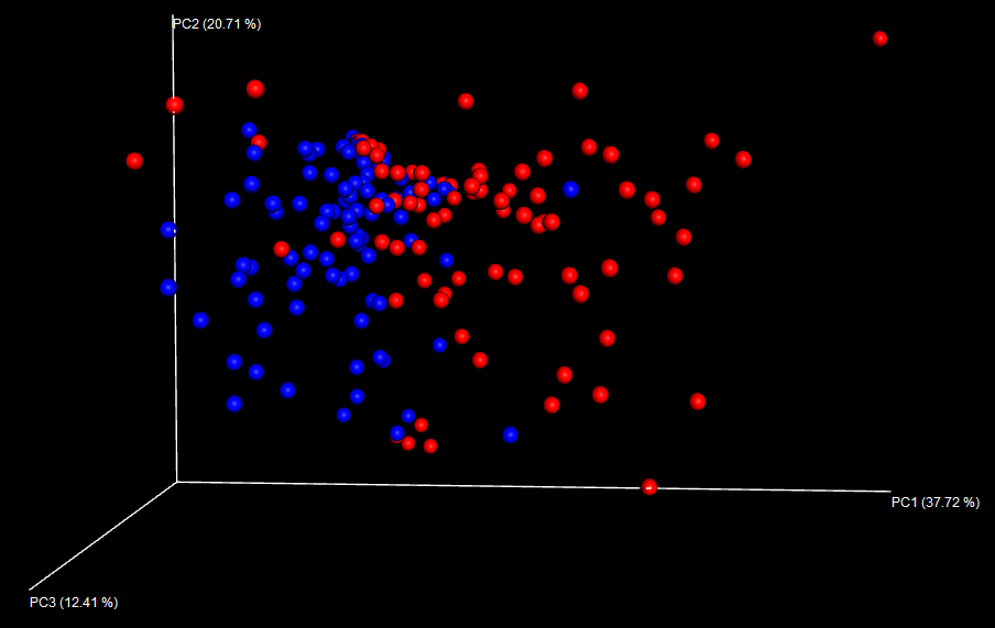
However, 3D plots don’t look great in a publication; it’s too easy to show a “nicer” pattern by rotating the plot, and you will always have one axis going into or coming out of the page which is difficult to interpret.

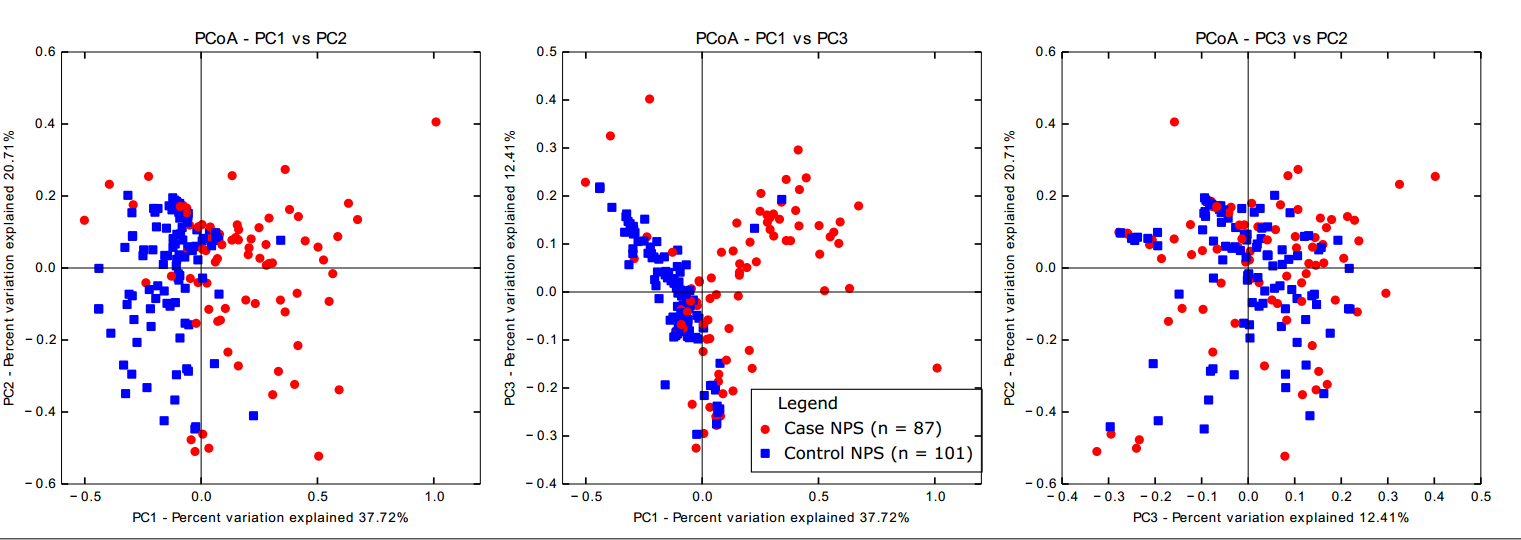
I created 2D plots from the 3D plots with a QIIME script, using the principal coordinates file (again, separately for NPS-NPS and case samples) and colouring by sample type:

make_2d_plots.py -i weighted_unifrac_pc.txt -m mapping_file_Runs1234.txt -o 2d_plots -b 'sample_type'

These plots look like this: they are separate files, but I put them together using Inkscape and added a legend.

Procrustes analysis

In addition to exploring the beta diversity, I also wanted to ensure that using raw instead of rarefied data would not lead me to different interpretations from the plot. Procrustes analysis is a transformation analysis where two coordinate matrices are optimally laid on top of each other so that they are as similar as possible. The purpose of this is to determine the similarity of the two matrices, indicating whether you would draw the same conclusions from a PCoA plot regardless of which you use.

I used Procrustes three times:

To compare raw to rarefied counts - does the lack of normalisation make a difference to the beta diversity conclusions?
To compare the middle ear fluid to middle ear rinse - does the sampling method of the middle ear change the conclusions?
To compare the left ear to the right ear - does it matter which is used?

To run Procrustes in QIIME, I needed the coordinate matrices generated from each member of the pair (i.e. raw/rarefied, fluid/rinse or left/right).

Raw/rarefied Procrustes

I generated the coordinates file using the beta_diversity_through_plots.py script above on the raw OTU table and again on one rarefied down to 1499 reads per sample. I did this twice; for the NPS/NPS beta diversity plot and again for the case samples plot.

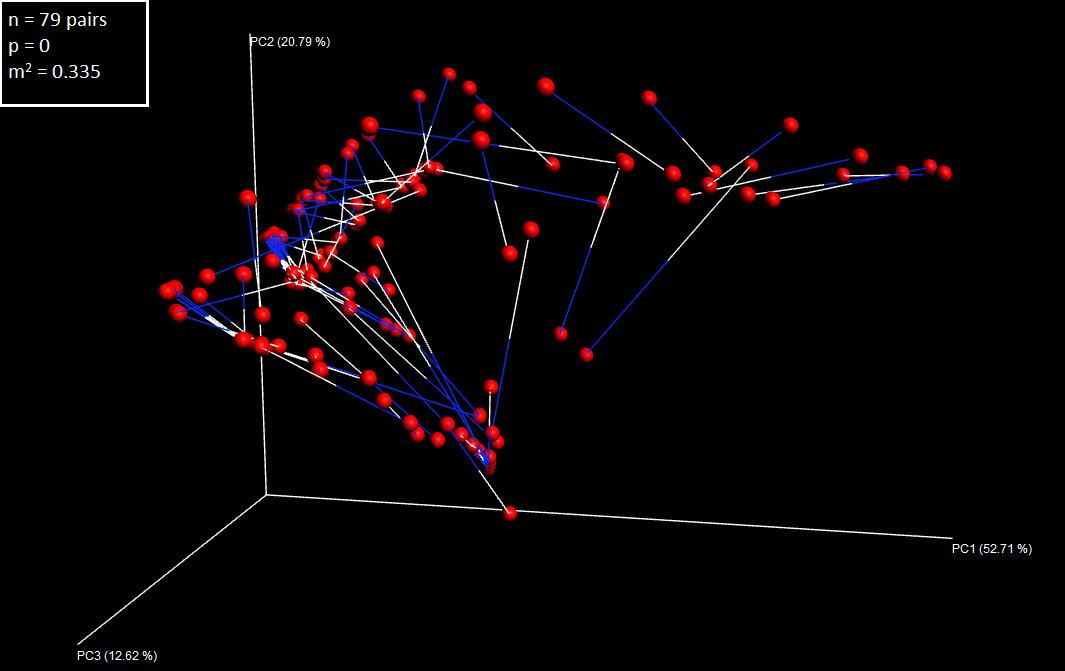
Then, for each, I did Procrustes analysis and made a 3D plot:

# Compare NPS matrix
transform_coordinate_matrices.py -i beta_nps_raw/weighted_unifrac_pc.txt,beta_regular_nps_1499/weighted_unifrac_pc.txt -r 999 -o procrustes/raw_rarefied_nps

# Make plot 
make_emperor.py -c -i procrustes/raw_rarefied_nps -o procrustes/raw_rarefied_nps/plots -m mapfile_Runs1234.txt

The output from transforming the matrix gives an m² value. This is a value representing how similar the matrices are; a minimum sum of squared distances, where a smaller value means the points are closer together. The -r flag is the number of permutations to determine a p-value for the m² value (i.e. the chance of seeing an m² at least this extreme).

The 3D plot looks much the same as the 3D plot for beta diversity, but it shows lines between the pairs of samples. You can see this better in the following image, because in my case the raw and rarefied matrices were extremely similar.

Fluid/rinse Procrustes

I first had to do a bit of data wrangling to subset the (raw) OTU table to fluids only and rinses only, but then only include pairs from the same ear of the same child.

By summarising the subsetted OTU table, I had a list of samples in it. I read these into R and chose my pairs:

# Get sample list
FR_pairs <- read.table("data/FR_list.txt", sep = "\t", header = F)
names(FR_pairs) <- "sample_ID"

# Convert the suffix to only "left" (L) or "right" (R) 
FR_pairs$newname <- gsub("F", "", FR_pairs$sample_ID)
# For rinses, this checks for strings of 8 characters in length and changes "RL" to "L" and "RR" to "R"
FR_pairs$newname <- ifelse(nchar(FR_pairs$newname) == 8, gsub("RL", "L", FR_pairs$sample_ID), FR_pairs$newname)
FR_pairs$newname <- ifelse(nchar(FR_pairs$newname) == 8, gsub("RR", "R", FR_pairs$sample_ID), FR_pairs$newname)

# Check that all assignments are correct
test1 <- as.character(FR_pairs$sample_ID)
test2 <- as.character(FR_pairs$newname)
test1 <- substr(test1, nchar(test1)-0, nchar(test1))
test2 <- substr(test2, nchar(test2)-0, nchar(test2))
#ifelse(test1 == test2, TRUE, FALSE)

# Remove IDs that only occur once; to ensure the list only contains pairs
tb.ID <- table(FR_pairs$newname)
appears.once <- names(tb.ID[tb.ID==1])
FR_pairs <- FR_pairs[!FR_pairs$newname %in% appears.once,]

# Export file with all paired fluid/rinse samples and "new" name: this file designates the pairs

#write.table(FR_pairs,"FR_map.txt", sep = "\t", row.names = F, col.names = F)

Then I needed to subset the OTU table to these samples.

# Export the sample IDs of chosen samples
samples <- FR_pairs$sample_ID
rinses1 <- as.character(samples[which(grepl("RR",samples))])
rinses2 <- as.character(samples[which(grepl("RL",samples))])
rinses <- c(rinses1,rinses2)
fluids <- as.character(samples[which(grepl("F",samples))])

#write.table(rinses,"rinses_keep.txt", sep = "\t", row.names= F, col.names = F)
#write.table(fluids,"fluids_keep.txt", sep = "\t", row.names= F, col.names = F)

Then in QIIME:

# Get rid of the quote marks given by R to character vectors
sed -i 's/\"//g' rinses_keep.txt
sed -i 's/\"//g' fluids_keep.txt
sed -i 's/\"//g' FR_map.txt

# Keep only the paired fluids in table
filter_samples_from_otu_table.py -i fluids.biom -o fluids_paired.biom --sample_id_fp fluids_keep.txt

# Keep only the paired rinses in table
filter_samples_from_otu_table.py -i rinses.biom -o rinses_paired.biom --sample_id_fp rinses_keep.txt

Finally, I do Procrustes on the fluid/rinse pairs using the sample pair map file I created:

# Run beta diversity on the two OTU tables
beta_diversity_through_plots.py -i fluids_paired.biom -m mapfile_Runs1234.txt -o beta_fluids -t rep_set.tre

beta_diversity_through_plots.py -i rinses_paired.biom -m mapfile_Runs1234.txt -o beta_rinses -t rep_set.tre

# Run Procrustes
transform_coordinate_matrices.py -i beta_fluids/weighted_unifrac_pc.txt,beta_rinses/weighted_unifrac_pc.txt -r 999 -o
transform -s FR_map.txt

Before I make the plot in Emperor, I need a version of the mapping file that has the new sample names. I modified the basic mapping file to have the new IDs, then made the plot:

# Make Procrustes plot 
make_emperor.py -c -i transform/ -m mapfile_FRpairs_procrustes.txt -o plots

The Procrustes plot looks like this (I have added the legend in Inkscape):

Left ear/right ear Procrustes

I took a similar approach to compare the left ear and right ear. I included both fluid and rinse samples but only paired fluid with fluid, and rinse with rinse.

I began by using the list of fluid and rinse samples from before:

# Get list of fluids and rinses
LR_pairs <- read.table("data/FR_list.txt", sep = "\t", header = F)
names(LR_pairs) <- "sample_ID"

# Convert suffix to "fluid" (F) or "rinse" (R)
LR_pairs$newname <- substr(LR_pairs$sample_ID, 1, nchar(as.character(LR_pairs$sample_ID))-1)

# Remove the samples that only occur once; these are only in one ear
tb.ID <- table(LR_pairs$newname)
appears.once <- names(tb.ID[tb.ID == 1])
LR_pairs <- LR_pairs[!LR_pairs$newname %in% appears.once, ]

# Export the list of pairs with "new" name
#write.table(LR_pairs, "left_right/LR_map.txt", sep = "\t", row.names = F, col.names = F)

Subsetted the OTU tables to these samples in QIIME:

samples <- LR_pairs$sample_ID
left <- as.character(samples[which(grepl("L", samples))])
right1 <- as.character(samples[which(grepl("FR", samples))])
right2 <- as.character(samples[which(grepl("RR", samples))])
right <- c(right1, right2)

#write.table(left, "left_keep.txt", sep = "\t", row.names = F, col.names = F)
#write.table(right, "right_keep.txt", sep = "\t", row.names = F, col.names = F)

# Remove the quote marks given by R
sed -i 's/\"//g' left_keep.txt
sed -i 's/\"//g' right_keep.txt
sed -i 's/\"//g' LR_map.txt

# Select the left samples from the fluids_rinses.biom table
filter_samples_from_otu_table.py -i ../fluid_rinse/fluids_rinses.biom -o left_paired.biom
--sample_id_fp left_keep.txt

# Select the right samples from the fluids_rinses.biom table
filter_samples_from_otu_table.py -i ../fluid_rinse/fluids_rinses.biom -o
right_paired.biom --sample_id_fp right_keep.txt

And ran the Procrustes analysis, again having altered the mapping file to contain the new sample IDs for plotting.

# Beta diversity on the separate tables
beta_diversity_through_plots.py -i left_paired.biom -m mapfile_Runs1234.txt -o beta_left -t rep_set.tre

beta_diversity_through_plots.py -i right_paired.biom -m mapfile_Runs1234.txt -o beta_right -t rep_set.tre

# Procrustes analysis 
transform_coordinate_matrices.py -i beta_left/weighted_unifrac_pc.txt,beta_right/weighted_unifrac_pc.txt -r 999 -o transform -s LR_map.txt

# Make plot
make_emperor.py -c -i transform -m mapfile_LRpairs_procrustes.txt -o plots