Correlation between OTUs with SparCC

Finally, I wanted to determine whether there were any strong correlations between the OTUs in any of the major sample types: particularly between these differentially abundant bacteria of interest.

The issue with correlations between bacteria in microbiome data is that the data is compositional; it describes the relative abundance of bactera, not absolute like if you were to determine bacterial load with qPCR. Each OTU contributes a proportion of reads that add up to 100% in each sample. The problem with searching for correlations here is that if there is an increase in one OTU, all of the other OTUs must decrease, and this ends up looking like a negative correlation between the increased OTU and everything else when this may not be the case.

A tool called SparCC determines correlations between OTUs taking this specific problem into account. This is what I have used, and it can be downloaded here. SparCC runs in Python so I used it on Linux.

Note that the samples should be independent; so for the MEF and MER I again took the Set 1/Set 2 approach making sure that any correlations were significant in both Sets to be considered true positive results.

Setting up data

First, I took the OTU table with low-depth samples and the taxonomy strings removed. I then created subsetted versions of the table for each sample type. As recommended in the SparCC paper I also removed OTUs with less than 2 reads on average in those samples.

I set up the OTU table for each sample type and exported it for use with SparCC.

This was straightforward for the NPS:

# Get full OTU table; no low-depth samples, no taxonomy
full.table <- read.table("data/final_otu_table_samples.txt", header = TRUE, check.names = F, sep = "\t", row.names = 1)

# Subset to case NPS
case.NPS <- full.table[, which(grepl("S1", names(full.table)))]
# Filter out OTUs that have less than 2 reads on average
case.NPS <- case.NPS[-which(rowMeans(case.NPS) < 2),]
#write.table(case.NPS, "case_NPS_filtered.txt", sep = "\t")

# Subset to control NPS
control.NPS <- full.table[, which(!grepl("MGO", names(full.table)))]
# Filter out low abundance OTus
control.NPS <- control.NPS[-which(rowMeans(control.NPS) < 2),]
#write.table(control.NPS, "control_NPS_filtered.txt", sep = "\t")

For the MEF and MER, I had to select one sample per child at random:

# Subset to fluids
fluids <- full.table[, which(grepl("F", names(full.table)))]

# To remove samples so that we have only one per child:

# List all the child ID numbers
fluid.pairs <- as.character(names(fluids))
fluid.pairs <- substr(fluid.pairs, 1, nchar(fluid.pairs)-2)

# Remove from the list the ones that appear once (don't need to select one at random)
f.tb.ID <- table(fluid.pairs)
f.appears.once <- names(f.tb.ID[f.tb.ID==1])
fluid.pairs <- fluid.pairs[!fluid.pairs %in% f.appears.once]

# List the IDs of children that have two fluids (one will be FL, one FR)
fluid.pairs <- unique(fluid.pairs)

# Assign at random "FL" or "FR" to the end - in this way I am selecting one at random
set.seed(42)
chosen.fluids <- sample(c("FL","FR"), length(fluid.pairs), replace = T)
chosen.fluids <- paste(fluid.pairs, chosen.fluids, sep = "")

# Subset the OTU table to these "chosen" fluids
chosen.fluids <- fluids[,which(names(fluids)%in% chosen.fluids)]
chosen.fluids$OTU <- rownames(chosen.fluids)

# List "unchosen" fluids (as opposites to "chosen" fluids)
unchosen.fluids <- names(chosen.fluids)
unchosen.fluids <- gsub("FL", "right", unchosen.fluids)
unchosen.fluids <- gsub("FR", "left", unchosen.fluids)
unchosen.fluids <- gsub("right", "FR", unchosen.fluids)
unchosen.fluids <- gsub("left", "FL", unchosen.fluids)

# Subset the OTU table to the "unchosen" fluids
unchosen.fluids <- fluids[,which(names(fluids)%in% unchosen.fluids)]
unchosen.fluids$OTU <- rownames(unchosen.fluids)

# List the sample IDs for fluids where there is only one available per child
unique.fluids <- names(fluids)
unique.fluids <- unique.fluids[!unique.fluids %in% names(chosen.fluids)]
unique.fluids <- unique.fluids[!unique.fluids %in% names(unchosen.fluids)]

# Subset the OTU table to these "unique" fluids
unique.fluids <- fluids[,which(names(fluids)%in% unique.fluids)]
unique.fluids$OTU <- rownames(unique.fluids)

# Create an OTU table of the "chosen" and "unique" fluids: Set 1
fluids.1 <- merge(chosen.fluids, unique.fluids, by = "OTU", sort = F)
rownames(fluids.1) <- fluids.1$OTU
fluids.1$OTU <- NULL

# Create an OTU table of the "unchosen" and "unique" fluids: Set 2
fluids.2 <- merge(unchosen.fluids, unique.fluids, by = "OTU", sort = F)
rownames(fluids.2) <- fluids.2$OTU
fluids.2$OTU <- NULL

# Remove low abundance OTUs and export for SparCC
fluids.1 <- fluids.1[-which(rowMeans(fluids.1) < 2), ]
fluids.2 <- fluids.2[-which(rowMeans(fluids.2) < 2), ]
#write.table(fluids.1, "fluids_1_filtered.txt", sep = "\t")
#write.table(fluids.2, "fluids_2_filtered.txt", sep = "\t")

For the fluids, I have 80 samples of which 33 are unique (child only had one analysable sample) and the rest (47) where an ear was chosen at random.

I repeated the same for the rinses:

# Subset to rinses
rinses <- full.table[, which(grepl("RL|RR", names(full.table)))]

# To remove samples so that we have only one per child:

# List all the child ID numbers
rinse.pairs <- as.character(names(rinses))
rinse.pairs <- substr(rinse.pairs, 1, nchar(rinse.pairs)-2)

# Remove from the list the ones that appear once (don't need to select one at random)
r.tb.ID <- table(rinse.pairs)
r.appears.once <- names(r.tb.ID[r.tb.ID==1])
rinse.pairs <- rinse.pairs[!rinse.pairs %in% r.appears.once]

# List the IDs of children that have two fluids (one will be FL, one FR)
rinse.pairs <- unique(rinse.pairs)

# Assign at random "RL" or "RR" to the end - in this way I am selecting one at random
set.seed(42)
chosen.rinses <- sample(c("RL","RR"), length(rinse.pairs), replace = T)
chosen.rinses <- paste(rinse.pairs, chosen.rinses, sep = "")

# Subset the OTU table to these "chosen" rinses
chosen.rinses <- rinses[,which(names(rinses)%in% chosen.rinses)]
chosen.rinses$OTU <- rownames(chosen.rinses)

# List "unchosen" rinses (as opposites to "chosen" rinses)
unchosen.rinses <- names(chosen.rinses)
unchosen.rinses <- gsub("RL", "right", unchosen.rinses)
unchosen.rinses <- gsub("RR", "left", unchosen.rinses)
unchosen.rinses <- gsub("right", "RR", unchosen.rinses)
unchosen.rinses <- gsub("left", "RL", unchosen.rinses)

# Subset the OTU table to the "unchosen" rinses
unchosen.rinses <- rinses[,which(names(rinses)%in% unchosen.rinses)]
unchosen.rinses$OTU <- rownames(unchosen.rinses)

# List the sample IDs for fluids where there is only one available per child
unique.rinses <- names(rinses)
unique.rinses <- unique.rinses[!unique.rinses %in% names(chosen.rinses)]
unique.rinses <- unique.rinses[!unique.rinses %in% names(unchosen.rinses)]

# Subset the OTU table to these "unique" rinses
unique.rinses <- rinses[,which(names(rinses)%in% unique.rinses)]
unique.rinses$OTU <- rownames(unique.rinses)

# Create an OTU table of the "chosen" and "unique" rinses: Set 1
rinses.1 <- merge(chosen.rinses, unique.rinses, by = "OTU", sort = F)
rownames(rinses.1) <- rinses.1$OTU
rinses.1$OTU <- NULL

# Create an OTu table of the "unchosen" and "unique" rinses" Set 2"
rinses.2 <- merge(unchosen.rinses, unique.rinses, by = "OTU", sort = F)
rownames(rinses.2) <- rinses.2$OTU
rinses.2$OTU <- NULL

# Remove low abundance OTUs and export for SparCC
rinses.1 <- rinses.1[-which(rowMeans(rinses.1) < 2), ]
rinses.2 <- rinses.2[-which(rowMeans(rinses.2) < 2), ]
#write.table(rinses.1, "rinses_1_filtered.txt", sep = "\t")
#write.table(rinses.2, "rinses_2_filtered.txt", sep = "\t")

I have 59 rinse samples where 5 are unique and the remaining 54 where two ears were available per child and one was chosen at random.

Now I have exported the OTU tables to perform the correlation analysis on.

Running SparCC

The steps in SparCC are straightforward:

Run SparCC on the OTU table to determine correlations in the data
Create 100 simulated datasets (the OTU table, shuffled randomly)
Calculate pseudo p-values by identifying how many of the 100 datasets produced a correlation with a magnitude at least as extreme as in the real data

Then I bring this data into R to produce correlograms. The code for the correlations in each sample type are below (all are the same).

Case NPS

Run SparCC on the samples for true correlation coefficients

# This averages the results over 20 estimates (defalt) of true fractions estimated from the counts with the Dirichlet distribution described in paper
python ~/bin/sparcc/SparCC.py case_NPS_filtered.txt -c case_NPS_sparcc.txt -v
case_NPS_cov_sparcc.txt

Run SparCC on bootstrapped datasets to generate pseudo p-values

# Default number of simulated datasets is 100: produces 100 files
python ~/bin/sparcc/MakeBootstraps.py case_NPS_filtered.txt -p simulated_case_NPS/ -t permuted_# 

mkdir boot_case_nps_corr
mkdir boot_case_nps_cov

# Then using the same defaults as before, run SparCC on each of these files
for i in `seq 0 99`; do python ~/bin/sparcc/SparCC.py simulated_case_NPS/permuted_$i -c boot_case_nps_corr/simulated_sparcc_$i.txt -v boot_case_nps_cov/simulated_sparcc_$i.txt >> case_NPS_boot_sparcc.log; done

Calculate the pseudo p-values

mkdir case_NPS_pvals

# One-sided p-values take into account the direction of correlation
python ~/bin/sparcc/PseudoPvals.py case_NPS_sparcc.txt boot_case_nps_corr/simulated_sparcc_#.txt 100 -o case_NPS_pvals/one_sided.txt -t one_sided

I now have the table of correlation coefficients between all pairs of OTUs and the table of pseudo p-values.

I load these into R and plot the correlation matrix:

library(corrplot)

## corrplot 0.84 loaded

# Bring in the correlation and p-value matrices
NPS.corr <- as.matrix(read.table("data/case_NPS_sparcc.txt", header = T, row.names = 1, sep = "\t"))
NPS.oneside <- as.matrix(read.table("data/case_NPS_one_sided.txt", header = T, row.names = 1, sep = "\t"))

# Combine the correlation and p-value matrices
NPS.1 <- list(NPS.corr, NPS.oneside)

# Plot the correlogram showing only significant correlations
corrplot(NPS.1[[1]], type = "lower", order = "FPC", p.mat = NPS.1[[2]], sig.level = 0.05, insig = "blank", tl.pos = "n", diag = F, cl.pos = "r")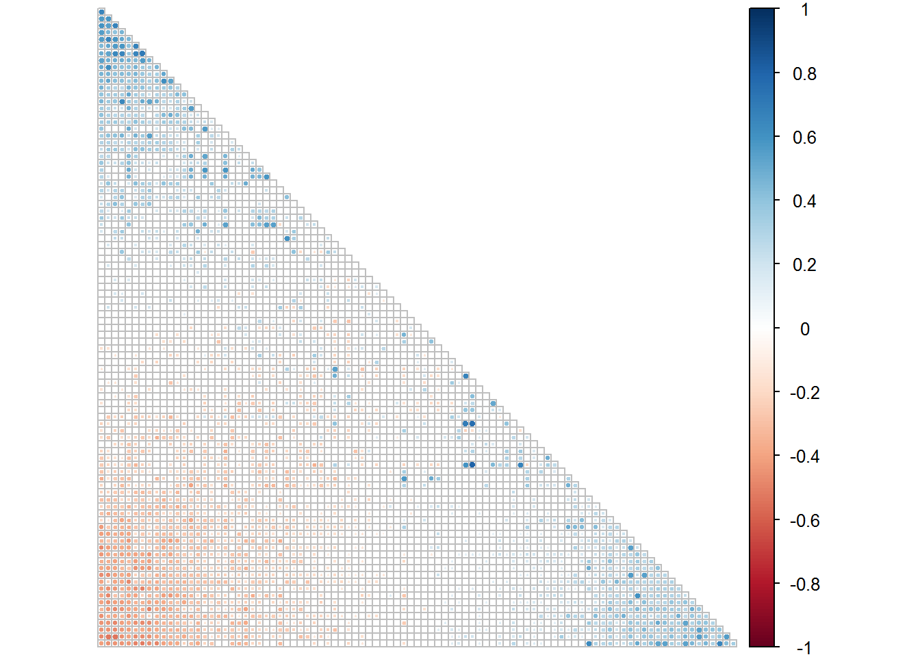

To get a list of all correlations from highest magnitude to lowest:

# List the correlation coefficients
NPS.all <- NPS.corr
NPS.all[lower.tri(NPS.all, diag = TRUE)] <- NA
NPS.all <- as.data.frame(as.table(NPS.all))
NPS.all <- na.omit(NPS.all)
names(NPS.all) <- c("Var1", "Var2", "Correlation")

# List the p-values
NPS.p <- NPS.oneside
NPS.p[lower.tri(NPS.p, diag = TRUE)] <- NA
NPS.p <- as.data.frame(as.table(NPS.p))
NPS.p <- na.omit(NPS.p)
names(NPS.p) <- c("Var1", "Var2", "p")

# Put the two in a table and export, sorting by correlation magnitude
NPS.out <- merge(NPS.all, NPS.p)
NPS.out <- NPS.out[order(-abs(NPS.out$Correlation)),]
#write.table(NPS.out, "caseNPS_all_correlations.txt", sep = "\t", row.names = F)

Control NPS

Run SparCC on the samples for true correlation coefficients

# Averaging the results over 20 estimates
python ~/bin/sparcc/SparCC.py controls_filtered.txt -c controls_sparcc.txt -v controls_cov_sparcc.txt

Run SparCC on bootstrapped datasets to generate pseudo p-values

# Produces 100 files
python ~/bin/sparcc/MakeBootstraps.py controls_filtered.txt -p simulated_controls/ -t permuted_#

mkdir boot_controls_corr
mkdir boot_controls_cov

# Run SparCC on each of these files
for i in `seq 0 99`; do python ~/bin/sparcc/SparCC.py simulated_controls/permuted_$i -c boot_controls_corr/simulated_sparcc_$i.txt -v boot_controls_cov/simulated_sparcc_$i.txt >> controls_boot_sparcc.log; done

Calculate the pseudo p-values

mkdir controls_pvals

# One-sided to account for direction of correlation
python ~/bin/sparcc/PseudoPvals.py controls_sparcc.txt boot_controls_corr/simulated_sparcc_#.txt 100 -o controls_pvals/one_sided.txt -t one_sided

Load the tables of correlation coefficients and p-values into R and plot the correlation matrix:

# Bring in the correlation and p-value matrices
controls.corr <- as.matrix(read.table("data/controls_sparcc.txt", header = T, row.names = 1, sep = "\t", check.names = F))
controls.oneside <- as.matrix(read.table("data/controls_one_sided.txt", header = T, row.names = 1, sep = "\t", check.names = F))

# Combine them
controls.1 <- list(controls.corr, controls.oneside)


# Plot significant correlations on correlogram
corrplot(controls.1[[1]], type = "lower", order = "FPC", p.mat = controls.1[[2]], sig.level = 0.05, insig = "blank", tl.pos = "n", diag = F, cl.pos = "r")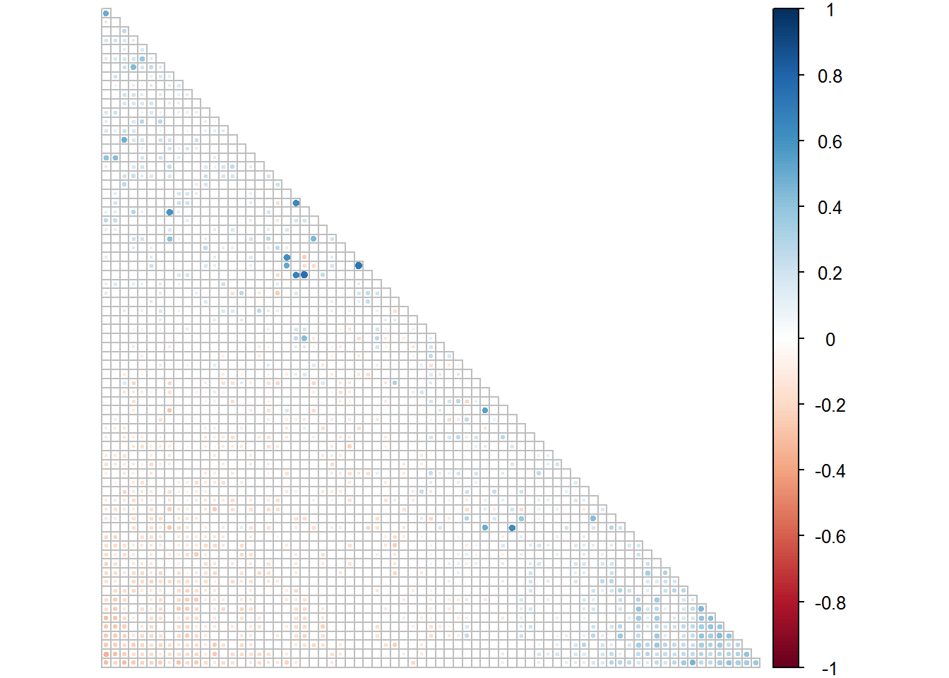

To output full list of correlation coefficients and p-values:

# List the correlation coefficients
controls.all <- controls.corr
controls.all[lower.tri(controls.all, diag = TRUE)] <- NA
controls.all <- as.data.frame(as.table(controls.all))
controls.all <- na.omit(controls.all)
names(controls.all) <- c("Var1", "Var2", "Correlation")

# List the p-values
controls.p <- controls.oneside
controls.p[lower.tri(controls.p, diag = TRUE)] <- NA
controls.p <- as.data.frame(as.table(controls.p))
controls.p <- na.omit(controls.p)
names(controls.p) <- c("Var1", "Var2", "p")

# Put them together and export, sorting by correlation magnitude
controls.out <- merge(controls.all, controls.p)
controls.out <- controls.out[order(-abs(controls.out$Correlation)),]
#write.table(controls.out, "controls_all_correlations.txt", sep = "\t", row.names = F)

MEF

Run SparCC on Set 1 and Set 2 of fluids for the true correlations

# Averaging over 20 estimates
python ~/bin/sparcc/SparCC.py fluids_1_filtered.txt -c fluids_1_sparcc.txt -v fluids_1_cov_sparcc.txt

python ~/bin/sparcc/SparCC.py fluids_2_filtered.txt -c fluids_2_sparcc.txt -v fluids_2_cov_sparcc.txt

Run SparCC on the simulated datasets for Set 1 and Set 2

# Creates 100 files each
python ~/bin/sparcc/MakeBootstraps.py fluids_1_filtered.txt -p simulated_fluids_1/ -t permuted_#

python ~/bin/sparcc/MakeBootstraps.py fluids_2_filtered.txt -p simulated_fluids_2/ -t permuted_#

mkdir boot_fluids_1_corr
mkdir boot_fluids_1_cov
mkdir boot_fluids_2_corr
mkdir boot_fluids_2_cov

# Run SparCC on each set of 100 files
for i in `seq 0 99`; do python ~/bin/sparcc/SparCC.py simulated_fluids_1/permuted_$i -c boot_fluids_1_corr/simulated_sparcc_$i.txt -v boot_fluids_1_cov/simulated_sparcc_$i.txt >> fluids_1_boot_sparcc.log; done

for i in `seq 0 99`; do python ~/bin/sparcc/SparCC.py simulated_fluids_2/permuted_$i -c boot_fluids_2_corr/simulated_sparcc_$i.txt -v boot_fluids_2_cov/simulated_sparcc_$i.txt >> fluids_2_boot_sparcc.log; done

Calculate the pseudo p-values for Set 1 and Set 2

mkdir fluids_1_pvals
mkdir fluids_2_pvals

python ~/bin/sparcc/PseudoPvals.py fluids_1_sparcc.txt boot_fluids_1_corr/simulated_sparcc_#.txt 100 -o fluids_1_pvals/one_sided.txt -t one_sided

python ~/bin/sparcc/PseudoPvals.py fluids_2_sparcc.txt boot_fluids_2_corr/simulated_sparcc_#.txt 100 -o fluids_2_pvals/one_sided.txt -t one_sided

Bring the files into R to generate correlogram:

# Read in Set 1 files
fluids1.corr <- as.matrix(read.table("data/fluids_1_sparcc.txt", header = T, row.names = 1, sep = "\t"))
fluids1.oneside <- as.matrix(read.table("data/fluids1_one_sided.txt", header = T, row.names = 1, sep = "\t"))

# Read in Set 2 files
fluids2.corr <- as.matrix(read.table("data/fluids_2_sparcc.txt", header = T, row.names = 1, sep = "\t"))
fluids2.oneside <- as.matrix(read.table("data/fluids2_one_sided.txt", header = T, row.names = 1, sep = "\t"))

# Combine the two matrices for each Set
fluids1.1 <- list(fluids1.corr, fluids1.oneside)
fluids2.1 <- list(fluids2.corr, fluids2.oneside)

# Plot correlogram for Set 1 (to be displayed in paper)
corrplot(fluids1.1[[1]], type = "lower", order = "FPC", p.mat = fluids1.1[[2]], sig.level = 0.05, insig = "blank", tl.pos = "n", diag = F, cl.pos = "r")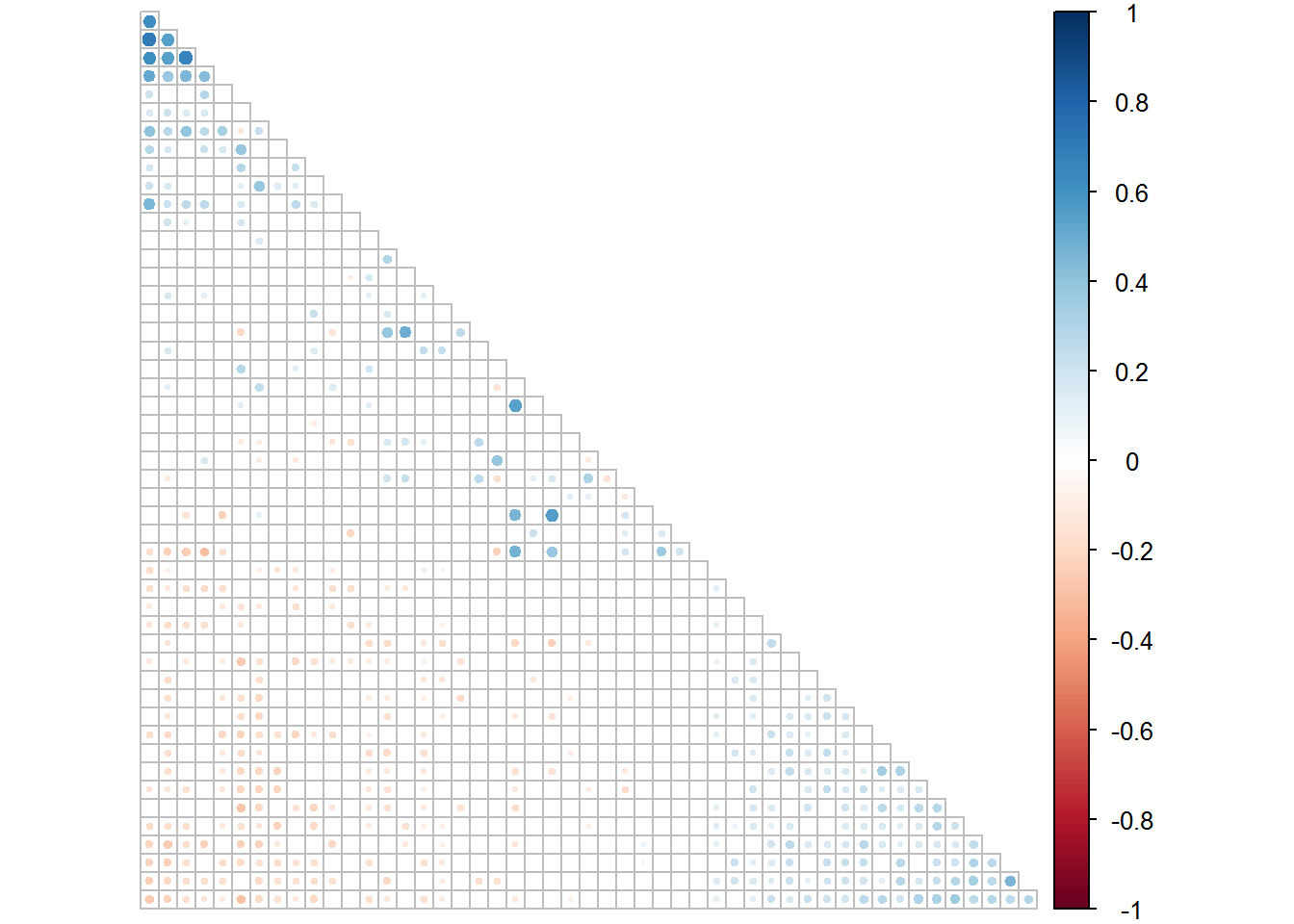

# Plot correlogram for Set 2
corrplot(fluids2.1[[1]], type = "lower", order = "FPC", p.mat = fluids2.1[[2]], sig.level = 0.05, insig = "blank", tl.pos = "n", diag = F, cl.pos = "r")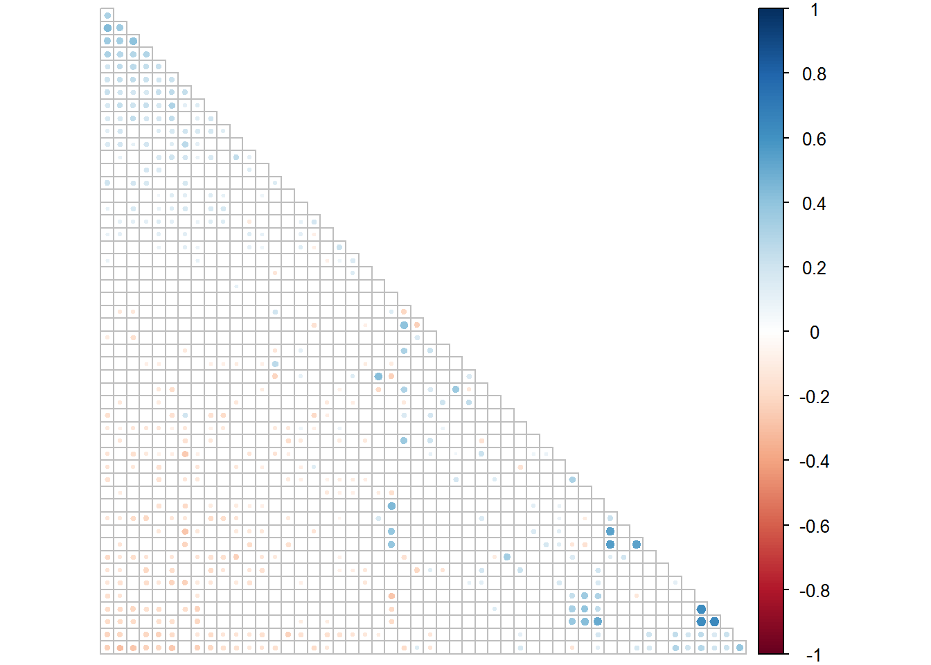

List all correlations and p-values for both Sets:

# List Set 1 correlations
fluids1.all <- fluids1.corr
fluids1.all[lower.tri(fluids1.all, diag = TRUE)] <- NA
fluids1.all <- as.data.frame(as.table(fluids1.all))
fluids1.all <- na.omit(fluids1.all)
names(fluids1.all) <- c("Var1", "Var2", "Correlation")

# List Set 1 p-values
fluids1.p <- fluids1.oneside
fluids1.p[lower.tri(fluids1.p, diag = TRUE)] <- NA
fluids1.p <- as.data.frame(as.table(fluids1.p))
fluids1.p <- na.omit(fluids1.p)
names(fluids1.p) <- c("Var1", "Var2", "p")

# Combine them into one table and export, sorting by correlation magnitude
fluids1.out <- merge(fluids1.all, fluids1.p)
fluids1.out <- fluids1.out[order(-abs(fluids1.out$Correlation)),]
#write.table(fluids1.out, "fluids1_all_correlations.txt", sep = "\t", row.names = F)

# List Set 2 correlations
fluids2.all <- fluids2.corr
fluids2.all[lower.tri(fluids2.all, diag = TRUE)] <- NA
fluids2.all <- as.data.frame(as.table(fluids2.all))
fluids2.all <- na.omit(fluids2.all)
names(fluids2.all) <- c("Var1", "Var2", "Correlation")

# List Set 2 p-values
fluids2.p <- fluids2.oneside
fluids2.p[lower.tri(fluids2.p, diag = TRUE)] <- NA
fluids2.p <- as.data.frame(as.table(fluids2.p))
fluids2.p <- na.omit(fluids2.p)
names(fluids2.p) <- c("Var1", "Var2", "p")

# Combine and export, sorting by correlation magnitude
fluids2.out <- merge(fluids2.all, fluids2.p)
fluids2.out <- fluids2.out[order(-abs(fluids2.out$Correlation)),]
#write.table(fluids2.out, "fluids2_all_correlations.txt", sep = "\t", row.names = F)

MER

Run SparCC on Set 1 and Set 2 of rinses for true correlations

# Averaging over 20 estimations
python ~/bin/sparcc/SparCC.py rinses_1_filtered.txt -c rinses_1_sparcc.txt -v rinses_1_cov_sparcc.txt

python ~/bin/sparcc/SparCC.py rinses_2_filtered.txt -c rinses_2_sparcc.txt -v rinses_2_cov_sparcc.txt

Run SparCC on 100 simulations each of Set 1 and Set 2 for p-values

# Produces 100 files each
python ~/bin/sparcc/MakeBootstraps.py rinses_1_filtered.txt -p simulated_rinses_1/ -t permuted_#

python ~/bin/sparcc/MakeBootstraps.py rinses_2_filtered.txt -p simulated_rinses_2/ -t permuted_#

mkdir boot_rinses_1_corr
mkdir boot_rinses_1_cov
mkdir boot_rinses_2_corr
mkdir boot_rinses_2_cov

# Run SparCC on the 100 files for each Set
for i in `seq 0 99`; do python ~/bin/sparcc/SparCC.py simulated_rinses_1/permuted_$i -c boot_rinses_1_corr/simulated_sparcc_$i.txt -v boot_rinses_1_cov/simulated_sparcc_$i.txt >> rinses_1_boot_sparcc.log; done

for i in `seq 0 99`; do python ~/bin/sparcc/SparCC.py simulated_rinses_2/permuted_$i -c boot_rinses_2_corr/simulated_sparcc_$i.txt -v boot_rinses_2_cov/simulated_sparcc_$i.txt >> rinses_2_boot_sparcc.log; done

Calculate the pseudo p-values for each Set

mkdir rinses_1_pvals
mkdir rinses_2_pvals

python ~/bin/sparcc/PseudoPvals.py rinses_1_sparcc.txt boot_rinses_1_corr/simulated_sparcc_#.txt 100 -o rinses_1_pvals/one_sided.txt -t one_sided

python ~/bin/sparcc/PseudoPvals.py rinses_2_sparcc.txt boot_rinses_2_corr/simulated_sparcc_#.txt 100 -o rinses_2_pvals/one_sided.txt -t one_sided

Bring into R to plot:

# Read in Set 1 matrices
rinses1.corr <- as.matrix(read.table("data/rinses_1_sparcc.txt", header = T, row.names = 1, sep = "\t"))
rinses1.oneside <- as.matrix(read.table("data/rinses1_one_sided.txt", header = T, row.names = 1, sep = "\t"))

# Read in Set 2 matrices
rinses2.corr <- as.matrix(read.table("data/rinses_2_sparcc.txt", header = T, row.names = 1, sep = "\t"))
rinses2.oneside <- as.matrix(read.table("data/rinses2_one_sided.txt", header = T, row.names = 1, sep = "\t"))

# Combine the correlation matrix and p-value matrix into a list
rinses1.1 <- list(rinses1.corr, rinses1.oneside)
rinses2.1 <- list(rinses2.corr, rinses2.oneside)

# Create correlogram for Set 1 (to display in paper)
corrplot(rinses1.1[[1]], type = "lower", order = "FPC", p.mat = rinses1.1[[2]], sig.level = 0.05, insig = "blank", tl.pos = "n", diag = F, cl.pos = "r")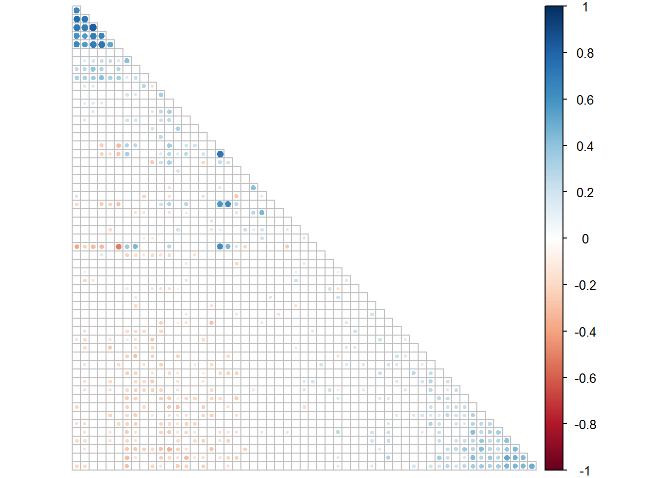

# Create correlogram for Set 2
corrplot(rinses2.1[[1]], type = "lower", order = "FPC", p.mat = rinses2.1[[2]], sig.level = 0.05, insig = "blank", tl.pos = "n", diag = F, cl.pos = "r")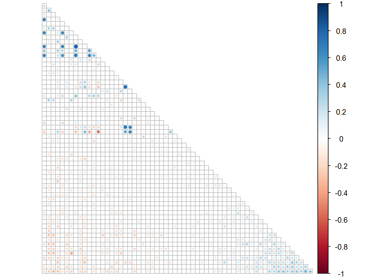

To list all correlations and p-values for both Sets:

# List correlations for Set 1
rinses1.all <- rinses1.corr
rinses1.all[lower.tri(rinses1.all, diag = TRUE)] <- NA
rinses1.all <- as.data.frame(as.table(rinses1.all))
rinses1.all <- na.omit(rinses1.all)
names(rinses1.all) <- c("Var1", "Var2", "Correlation")

# List p-values for Set 1
rinses1.p <- rinses1.oneside
rinses1.p[lower.tri(rinses1.p, diag = TRUE)] <- NA
rinses1.p <- as.data.frame(as.table(rinses1.p))
rinses1.p <- na.omit(rinses1.p)
names(rinses1.p) <- c("Var1", "Var2", "p")

# Put both lists into a table and export, sorting by correlation magnitude
rinses1.out <- merge(rinses1.all, rinses1.p)
rinses1.out <- rinses1.out[order(-abs(rinses1.out$Correlation)),]
#write.table(rinses1.out, "rinses1_all_correlations.txt", sep = "\t", row.names = F)

# List correlations for Set 2
rinses2.all <- rinses2.corr
rinses2.all[lower.tri(rinses2.all, diag = TRUE)] <- NA
rinses2.all <- as.data.frame(as.table(rinses2.all))
rinses2.all <- na.omit(rinses2.all)
names(rinses2.all) <- c("Var1", "Var2", "Correlation")

# List p-values for Set 2
rinses2.p <- rinses2.oneside
rinses2.p[lower.tri(rinses2.p, diag = TRUE)] <- NA
rinses2.p <- as.data.frame(as.table(rinses2.p))
rinses2.p <- na.omit(rinses2.p)
names(rinses2.p) <- c("Var1", "Var2", "p")

# Combine and export, sorting by correlation magnitude
rinses2.out <- merge(rinses2.all, rinses2.p)
rinses2.out <- rinses2.out[order(-abs(rinses2.out$Correlation)),]
#write.table(rinses2.out, "rinses2_all_correlations.txt", sep = "\t", row.names = F)

Thus ends the analyses on my 16S rRNA gene amplicon data.