Pre-processing reads

To start, I downloaded the files from the sequencing centre onto the analysis server with wget as instructed in the notification email.

The following steps were applied separately to the files from each sequencing run.

I validated the files with the checksums file that was provided with them:

md5sum -c checksums.md5

and then decompressed the files and renamed the directory to raw_data/

gunzip *.fastq.gz
cd ../
mv <old_name> raw_data/

FastQC overall quality check

I like to check the overall quality of the data to make sure that nothing horrendous happened to the sequencing run, and I do this with FastQC. I made a shell script that contains the following:

#!/bin/bash

# Pool all forward and all reverse reads separately to assess quality in fastqc
mkdir fastqc_check
cat raw_data/*_R1.fastq >> fastqc_check/forward_reads.fastq
cat raw_data/*_R2.fastq >> fastqc_check/reverse_reads.fastq
mkdir fastqc_check/forward_reads
mkdir fastqc_check/reverse_reads

# Run fastqc on these files
fastqc fastqc_check/forward_reads.fastq -o fastqc_check/forward_reads
fastqc fastqc_check/reverse_reads.fastq -o fastqc_check/reverse_reads

This allows me to look at the overall quality of the forward reads and the reverse reads (which are usually worse), per run.

I made this shell script executable

chmod +x fastqc.sh

And put it in my PATH by placing it in my ~/bin directory and adding the following line to ~/.bashrc:

export PATH=$HOME/bin:$PATH

Note that these steps are applied to any script or executable file that I use.

I run it from the directory above raw_data/:

fastqc.sh

The output in fastqc_check/ provides a HTML file with all of the FastQC stats. The one I am interested in is the plot of read quality:

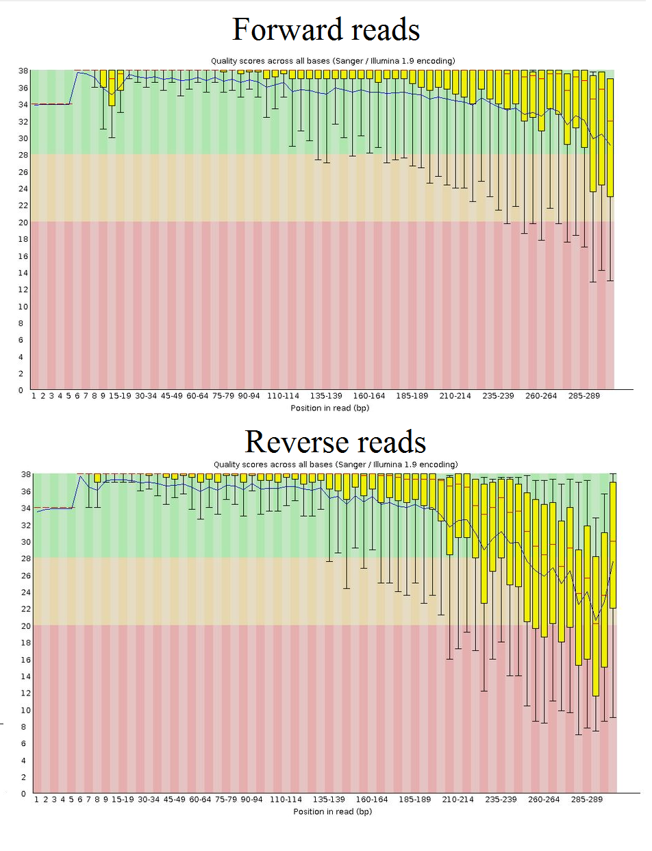
This is an example of the quality from one of the sequencing runs. Notice that the read quality drops towards the end of the reads, particularly in the reverse reads; this is normal. The advantage of merging these paired-end reads later is that the quality can be improved (if overlapping bases are the same in both reads, there is a higher likelihood that the correct base was called) so there is no need for trimming here.

Preparing to stitch the reads

The next step is to stitch (or merge) the paired-end reads. The sequenced region (V3/V4) should be around 465 bp long (by E. coli numbering). Because we sequenced 600 bp in total (300 bp from each end), there should be some overlap in the middle that can be used to align the read pairs and create a merged read.

‘Renaming’ files

Initially, these files were a bit messy to work with because the filenames were so long, e.g. MGO_067_S1_AN5R5_CGAGGCTG-AAGGAGTA_L001_R1.fastq MGO_067_S1_AN5R5_CGAGGCTG-AAGGAGTA_L001_R2.fastq

To make things easier, I used a Perl script written by a colleague to create symbolic links for each file in the directory above raw_data so they looked like this instead: MGO067S1_R1.fastq MGO067S1_R2.fastq

Using symbolic links preserves the original files. The purpose was to have no other underscores before _R1 so that USEARCH can elegantly relabel the reads with only the sample ID.

Setting length restrictions

As a form of quality filtering, I decided to restrict the final length of sequences when merging the paired end reads. This removes anything that is too long or too short (and would therefore be a poor read or a poor merge). As I initially didn’t know exactly how long these reads should be, I tested by merging first and looking at where the majority of the reads fell. This does not output the merged reads; just a log file.

mkdir -p merge_test
usearch -fastq_mergepairs *_R1.fastq -fastq_merge_maxee 1 -relabel @ -report merge_test/merge_test.log

This command automatically finds the matching _R2.fastq pair for each _R1.fastq file, filters out reads with an expected error value of greater than 1 (quality filtering), relabels each read with the filename prefix and gives me some output to look at.

By checking the log, I can see where most of the reads fall:

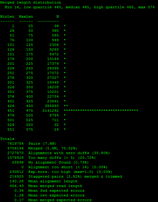
I actually repeated this step once more, restricting the lengths further:

usearch -fastq_mergepairs *_R1.fastq -fastq_minmergelen 450 -fastq_maxmergelen 480 -fastq_merge_maxee 1 -relabel @ -report  merge_test/merge_test2.log 

And checked the log again. Based on where most of them fell, I decided to throw out reads that were not between 440 bp - 470 bp. For each sequencing run I examined the lengths again to ensure that this setting remained appropriate, but I did apply the same restrictions to the data from each run for consistency.

Stitching the reads

Now that I have worked out the ideal length restrictions for my reads, I merge the forward and reverse reads together with expected error filtering to remove low quality reads.

Expected error filtering is explained here: http://drive5.com/usearch/manual/exp_errs.html

Note that in the UPARSE documentation it is now recommended to merge without quality filtering, then remove primers, then quality filter in a separate step.

mkdir -p usearch_merge
usearch -fastq_mergepairs *_R1.fastq -fastq_minmergelen 440 -fastq_maxmergelen 470 -fastq_merge_maxee 1 -relabel @ -report usearch_merge/merge.log -fastqout usearch_merge/merged.fastq -tabbedout usearch_merge/detail_pairs.log

This file merged.fastq contains the high quality set of reads that will be used for picking OTUs. However, most of the reads thrown out by the quality filtering will actually be good enough to map to an OTU and it is ideal to include as many reads as possible. So, separately, I merge all of the raw reads again but this time without the expected error filtering.

usearch -fastq_mergepairs *_R1.fastq -fastq_minmergelen 440 -fastq_maxmergelen 470 -relabel @ -report usearch_merge/merge_nofilter.log -fastqout usearch_merge/merged_nofilter.fastq -tabbedout usearch_merge/detail_pairs_nofilter.log

I then recompressed the raw data to save space on the server.

cd raw_data
gzip *.fastq

Creating a QIIME mapping file

Before I moved on, I created a QIIME mapping file which I also used outside of QIIME. This is the file that relates each sample to all of the information you have about that sample.

The bare minimum file contains the headings #SampleID (the # is important), BarcodeSequence, LinkerPrimerSequence and Description. In between the last two, you can have as many columns as you like containing other information.

In our study, I included all of the information from our questionnaire (things like age, gender, recent antibiotic use, etc.) as well as sample type and a column named ReversePrimer. This column was included for the removal of amplicon primers from the reads; described in the following section. I put the sequence of the reverse amplicon primer here, with the forward primer in LinkerPrimerSequence, both in 5’ to 3’ orientation. Because the Illumina adapters and unique indexes are removed by the MiSeq, I left BarcodeSequence blank and copied the sample ID into the Description field.

I made this file initially in Excel, saved it as a tab-delimited text file and used R to add most of the questionnaire data (dealing with data frames was easier than multiple Excel files).

I then validated this mapping file in QIIME (i.e. QIIME checks that it is formatted correctly). I pass the -b flag to ignore the empty BarcodeSequence column, and -j to designate the column to demultiplex by in the absence of unique barcodes. (This seems to have been designed with non-demultiplexed sequencing runs in mind; the MiSeq will demultiplex for you, giving you separate files for each sample.)

Within the QIIME environment:

validate_mapping_file.py -m mapfile_Run_X.txt -o mapfile_Run_X_check -b -j Description

Note that I am still doing this once per sequencing run at this point. I also created one mapping file containing all samples for use downstream.

The output specifies what is wrong (if anything) with the file; I made sure the file was okay before proceeding.

Stripping amplicon primers

I now move back to processing the reads; I have merged the paired-end reads with and without quality filtering.

The sequencing reads should only contain biological sequence. The MiSeq removes the Illumina adapter sequences and anything that comes before/after it, so these reads are fine. However, the amplicon primers should also be removed as they are prone to errors. Note that it is now recommended to do this prior to quality filtering.

Because the read length is still slightly variable, I did not want to trim a fixed number of bases off the ends. Instead, I used a custom script written by Tony Walters (thank you!) to detect and remove amplicon primer sequences specified in the mapping file:

strip_primers_fastq.py ~/MGO_analysis/mapping_files/mapfile_RunX.txt merged.fastq merged_noprimers.fastq strip_primers_log.txt
strip_primers_fastq.py ~/MGO_analysis/mapping_files/mapfile_RunX.txt merged_nofilter.fastq merged_nofilter_noprimers.fastq strip_primers_nofilter_log.txt

It is important that the error-filtered reads (merged.fastq) and the non-error filtered reads (merged_nofilter.fastq) are treated the same, so I applied this script to both files. The log file describes how many primers were detected and removed.

Dereplication

Dereplication is the process where all of the quality-filtered sequences are collapsed into a set of unique reads, which are then clustered into OTUs.

Converting to FASTA

Firstly, I don’t need the quality information anymore so I converted the merged_noprimers.fastq and merged_nofilter_noprimers.fastq files for each sequencing run to FASTA. I remember this step taking a while (a few hours) as it doesn’t seem to be able to run in parallel.

In the QIIME environment:

convert_fastaqual_fastq.py -f merged_noprimers.fastq -c fastq_to_fastaqual
convert_fastaqual_fastq.py -f merged_nofilter_noprimers.fastq -c fastq_to_fastaqual

I now combine the quality-filtered files from each sequencing run.

I concatenated the high-quality FASTA files for each sequencing run, replacing the filenames with the path to the merged_noprimers.fna file for each run:

cat <Run1>.fna <Run2>.fna <Run3>.fna <Run4>.fna >> Runs1234_filtered.fna

Reducing memory usage: dereplicating in parts

(Thanks to Ghislaine Platell for this tip)

This combined file was too large for the command to run due to the memory limitations of USEARCH 32-bit. To reduce memory usage I split the file into parts. This made the dereplication step a lot slower, but in my experience USEARCH was very fast regardless.

The file needs to be under ~2GB to use less than the maximum 4GB of memory. I looked at the size of the file, determined how many parts it would need to be split into, and then chose to split by number of lines. The number had to be divisible by 6 because each sequence (plus the FASTA header) took up 6 lines.

split -l 8400000 Runs1234_filtered.fna

This number of course depends on the file itself. As a sanity check, I looked at the head and tail of each part (named by default xaa, xab etc.) to confirm that I hadn’t split sequences across files.

To dereplicate the sequences, I used USEARCH’s -derep_fullength command. (Note that is is now deprecated; use -fastx_uniques instead.) To end up with a final, single file with only unique sequences I ran the derep command on each part, combined the outputs, and then ran derep on this file (which was now small enough).

usearch -derep_fulllength xaa - fastaout xaa_uniques.fasta -sizeout -relabel uniq_ -threads 8

I repeated the above on all xa- parts. The -sizeout option records the number of times that unique read occurs, which is important for the actual read counts to be retained. The FASTA headers are also relabelled with uniq_. Note that at this point, I have lost the information on which reads come from which sample: this isn’t a problem, because I only use this file to create the representative set of OTUs. The merged_nofilter_noprimers.fna data is used to assign OTUs to sequences and that file still has this information.

After derepping the parts, I combine and derep the whole;

cat xaa_uniques.fasta xab_uniques.fasta <etc> >> Runs1234_uniques_split.fna

usearch -derep_fulllength Runs1234_uniques_split.fna -fastaout Runs1234_uniques.fna -sizeout -sizein -relabel uniq_ -threads 8

Note that again I use -sizeout, but I also use -sizein so the command recognises the counts for each unique read that are already in the headers. This way the total count of each read is retained.

This last file is the full set of unique sequences.

Remove human reads

This step is optional. In our particular data set, my modifications to the PCR protocol allowed us to amplify out of our low biomass samples (many samples yielded under 5 ng/ul DNA at extraction), but this resulted in a lot of off-target amplification from human DNA. This meant that there was actually quite a bit of human sequence in the data (my preliminary analysis showed some OTUs BLASTing to the human genome) so I decided that it was worth filtering these out.

For this step, I used DeconSeq. The web version was not accepting submissions at the time I ran this (and still isn’t as of April 2017) so I downloaded the standalone version.

I followed the documentation to index the human genome (I used build 38, patch 2) with the version of bwa that was included with the tool (it wouldn’t work for me with the latest version of bwa). I filtered out the human sequences from the set of uniques using the default values of coverage and identity:

perl deconseq.pl -f Runs1234_uniques.fna -dbs hsref -c 90 -i 94

This outputs a ‘clean’ FASTA file and a ‘cont’ FASTA file. (Clean - human sequences removed, contaminated - the sequences that were removed). The clean file is what I continued with.

OTU clustering

Now I have my clean set of quality filtered unique sequences, the next step is OTU picking (or clustering). This step refers to aligning the sequences to each other to determine representative OTU sequences. Sequences that are at least 97% identical (by default; not recommended to change) are clustered together as an OTU.

This command uses the UPARSE algorithm. It also discards sequences that it identifies as chimeric (erroneous sequences that contain bases from more than one organism; artefactually joined into one read) so there is no need to run a separate chimera-checking step.

I take the high quality, human-cleaned file and cluster OTUs:

usearch -cluster_otus Runs1234_uniques_nohuman.fasta -otus otu_rep_set.fna -uparseout cluster_otus_detail.up -minsize 2 -sizeout -sizein -relabel OTU -log cluster_otus.log

The -otus flag designates the output file of representative OTU sequences. -uparseout is a kind of log that shows how each sequence was classified. The -minsize flag, when set to 2, discards singletons; reads that occur only once are likely to be errors. This ensures that the rep set is of high quality; but when I align the raw reads to this in the next step, the singletons are included and will map to an OTU if they are good enough. Again, -sizeout and -sizein hold the read counts (though I think they become meaningless or mean something different in the rep set output; not certain) and the sequences are renamed with “OTU” so they will be OTU1, OTU2 etc.

The log file will print the number of OTUs found and the number of chimeric sequences discarded.

Creating OTU tables

I have now created a file with a set of sequences where each represents a separate OTU. This was generated from a high quality set of my original reads; I have determined which OTUs are present in my data. Now, I need to go back to those merged but not quality-filtered reads and assign an OTU to each one. To do this, I align these reads to the OTU representative set.

This is the set of reads that were treated in the same way as the high quality set (paired-end reads merged with 440-470 bp cutoff, amplicon primers removed) but they did not undergo expected error filtering in the merging step. This is my merged_nofilter_noprimers.fna file from earlier; one for each sequencing run.

Here I combine the unfiltered reads from each sequencing run.

Just like the high quality sequences, I concatenate the reads from each sequencing run together and then split this file so it is small enough to run the command. Again this splitting is based on the size and the number of lines.

cat <Run1>.fna <Run2>.fna <Run3>.fna <Run4>.fna >> Runs1234_nofilter.fna

split -l 8700000 Runs1234_nofilter.fna

I now align each part to the OTU rep set, creating an OTU table for each:

usearch -usearch_global xaa.fna -db otu_rep_set.fna -strand plus -id 0.97 -otutabout otu_table.txt -biomout otu_table_xaa.biom

xaa.fna is the first part; I repeated this step for each part.

The ID parameter (set to 0.97) means that if a read is at least 97% identical to an OTU representative sequence, it will be assigned that OTU.

The standard output will show the percentage of reads that mapped to an OTU. Any human sequences in this read set (I did not run DeconSeq on these unfiltered reads) should be filtered out here as they will not map to an OTU.

I have one OTU table for each split set of reads; to make my full OTU table, I simply merge these OTU tables with a QIIME script:

merge_otu_tables.py -i otu_table_xaa.biom,otu_table_xab.biom -o merged_otu_table.biom

Assigning taxonomy to the OTU table

My full OTU table is a matrix of counts for each OTU by sample. However, I don’t yet know what these OTUs actually are; I need to assign taxonomy to them.

I am using the SILVA database (v123) designed for use with QIIME. I am switching from QIIME’s default GreenGenes because the latest SILVA release was more recent at the time of analysis. Importantly, GreenGenes misclassifies Dolosigranulum as Alloiococcus and both genera were actually very important in this study.

Again, within QIIME:

# Assign taxonomy to the reads
assign_taxonomy.py -i otu_rep_set.fna -t ~/databases/SILVA123_QIIME_release/taxonomy/16S_only/97/taxonomy_7_levels.txt -r ~/databases/SILVA123_QIIME_release/rep_set/rep_set_16S_only/97/97_otus_16S.fasta -o uclust_assigned_taxonomy

# Remove the size annotations from this file because the next step expects semicolons to separate taxonomy strings (and we don't need the size annotation anymore) 
sed 's/;size=[0-9]*;//g' uclust_assigned_taxonomy/otu_rep_set_tax_assignments.txt > uclust_assigned_taxonomy/tax_assignments_fixed.txt

# Add the taxonomy strings to the OTU table
biom add-metadata -i merged_otu_table.biom -o merged_otu_table_w_tax.biom --observation-metadata-fp uclust_assigned_taxonomy/tax_assignments_fixed.txt --sc-separated taxonomy --observation-header OTUID,taxonomy

Now I have an OTU table that contains taxonomic names.

Cleaning up the OTU table and creating a phylogenetic tree

The final part of this pre-processing segment of analysis is filtering this OTU table and creating a phylogenetic tree for downstream analyses.

Firstly, I filtered out any OTUs whose sequences did not align to the pre-aligned SILVA core set with PyNAST (within QIIME). This step is done by default in the QIIME OTU picking workflows (something I didn’t use, but decided to follow in this regard).

# Remove the size annotations and semicolons from the rep set: seemed to cause problems
sed 's/;size=[0-9]*;//g' otu_rep_set.fna > otu_rep_set_nosize.fna

# Align the sequences to the SILVA core set with PyNAST
parallel_align_seqs_pynast.py -i otu_rep_set_nosize.fna -t ~/databases/SILVA123_QIIME_release /core_alignment/core_alignment_SILVA123.fasta -o pynast_aligned_seqs -O 8

# Filter the alignment to remove gaps
filter_alignment.py -i otu_rep_set_nosize_aligned.fasta

# Remove OTUs that didn't align from the OTU table
filter_otus_from_otu_table.py -i merged_otu_table_w_tax.biom -o merged_otu_table_w_tax_no_pynast_failures.biom -e pynast_aligned_seqs/otu_rep_set_nosize_failures.fasta

OTUs below an abundance of 0.005% are probably errors or chimeras that have escaped the filtering this far, according to Bokulich et al. so I removed these OTUs with a QIIME script.

# Filter OTUs at < 0.005% abundance
filter_otus_from_otu_table.py -i merged_otu_table_w_tax_no_pynast_failures.biom -o final_otu_table_all.biom --min_count_fraction 0.00005

# Summarise the table to see how many reads per sample we have
biom summarize-table -i final_otu_table_all.biom -o biom_summaries/final_otu_table_all_summary.txt

I have named this the “final” OTU table because this is now the OTU table from which all of my other analysis stems. Depending on what I need, I filter this table further by sample type, or I remove the positive and negative sequencing controls, or remove samples with a low read count (1499 was my arbitrary threshold in this study). This is easily done with the QIIME script filter_samples_from_otu_table.py.

Lastly, I create a phylogenetic tree for downstream analysis; the UniFrac metric uses it for beta diversity calculations, as does the phylogenetic alpha diversity metric Faith’s PD. The tree is created from the aligned and filtered OTU rep set that I just made:

make_phylogeny.py -i otu_rep_set_nosize_aligned_pfiltered.fasta -o ../rep_set.tre -l ../make_phylogeny.log

The OTU table and the phylogenetic tree are the major files that I will need in further analyses; this is the end of the data pre-processing.