Exploring taxonomy

Summarising taxa

Now that I have the OTU table, the first thing I want to do is look at which bacteria we have in the samples! I have done this by summarising the taxonomy in the form of bar charts, though this information as a table is more detailed.

Usually, there will be multiple OTUs with the same taxonomy assignment. These may be spurious (perpetuated errors, chimeras) or could be different species where the sequence identity is less than 97% but the genus-level taxonomy is the same. Some OTUs may also contain multiple species if they are more than 97% identical. Summarising the taxonomy in QIIME groups the OTUs by their taxonomy name to give a general overview of what’s present in the samples.

I was more interested in summarising by sample type than by individual samples, so I included this in the taxa summary step.

At this point, I have filtered my input OTU table, named otu_table.biom here so that it contains only samples (not positive or negative sequencing controls) with at least 1499 reads by using filter_samples_from_otu_table.py.

summarize_taxa_through_plots.py -i otu_table.biom -o sample_type_plots
-m mapfile_Runs1234.txt -c sample_type

From this output, I didn’t take the plots but the file it produced: sample_type_otu_table_L6.txt as I wanted to make more customisable plots in R. I altered the taxonomy in this file by removing everything before D_5, which designates genus, so it only contained readable genus names instead of the entire taxonomy string. I then made the plot in R:

data <- read.table("data/sample_type_otu_table_L6.txt", header = T, sep = "\t")

# Collapse anything with a total of less than 1.0% into "Other" before plotting (just to have a concise legend) 
data$taxa <- ifelse(rowSums(data[,2:6]/5) < 0.01, "Other", as.character(data$taxa))
other <- data[which(data$taxa == "Other"),]
other <- colSums(other[2:6])
data <- data[-which(data$taxa == "Other"),]
other <- append(other, "Other (49 other taxa)")
names(other) <- c("control", "rinse", "fluid", "NPS", "canal", "taxa")
other <- other[c(6,1:5)]
data <- rbind(data,as.data.frame(t(other)))

# Make all numeric
for (i in 2:length(data)) {
  data[,i] <- as.numeric(data[,i])
}

# Change to long format
library(reshape2)
datam <- melt(data)
datam$value <- datam$value * 100
datam$taxa <- factor(datam$taxa, levels = data$taxa)

# To label the axis ticks properly, use mapvalues (plyr):
library(plyr)
datam$sample_type_labels <- mapvalues(datam$variable, c("NPS", "control", "fluid", "rinse", "canal"), c("Case NPS\n(n = 87)", "Control NPS\n(n = 101)", "MEF\n(n = 127)", "MER\n(n = 113)", "Ear canal\n(n = 53)"))

# Reorder the factor so the NPS are next to each other
datam$sample_type_labels <- factor(datam$sample_type_labels, levels = c("Case NPS\n(n = 87)", "Control NPS\n(n = 101)", "MEF\n(n = 127)", "MER\n(n = 113)", "Ear canal\n(n = 53)"))

# Plot as a bar graph; keep the ggplot colours but specify them
library(scales)
library(ggplot2)
set.seed(4564)

n <- length(levels(datam$taxa))
cols <- hue_pal(h = c(0,360) + 15, c = 100, l = 65, h.start = 0, direction = 1)(n)[c(11,7,1,3,5,9,2,6,4,8,10)]
ggplot(datam, aes(x = sample_type_labels, y = value)) + 
    geom_bar(aes(fill = taxa), stat = "identity") +
    labs(x = "Sample type", y = "Relative abundance (%)") +
    scale_fill_manual(name = "Genus", values = cols)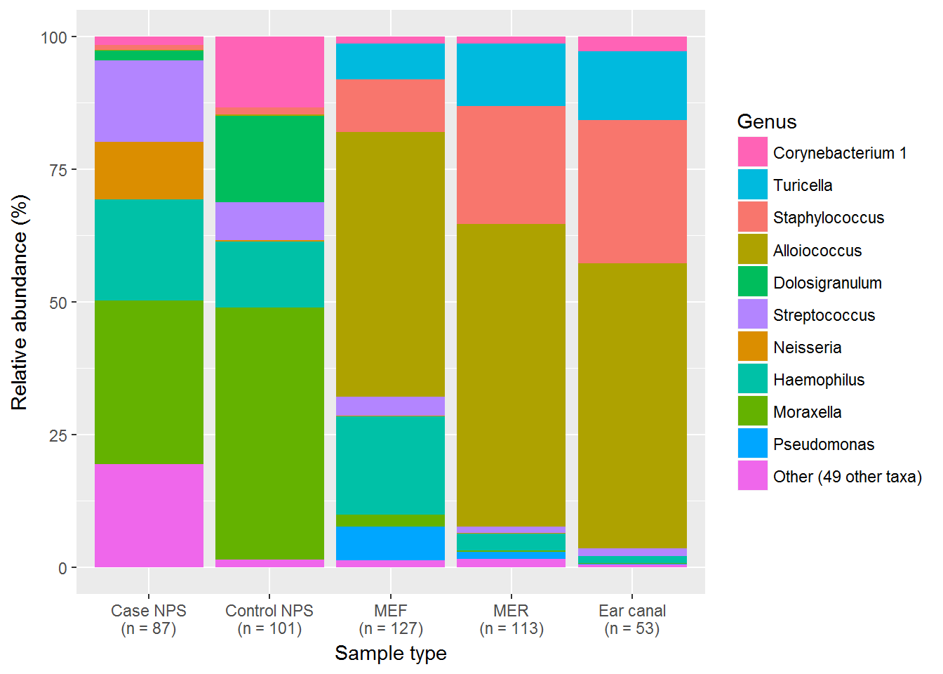

This is a nice overview of the major genera in each sample type. But, as it can be difficult to compare by eye, the table is more useful to look at.

taxa	control	rinse	fluid	NPS	canal
Corynebacterium 1	13.3041203	1.3356343	1.3548518	1.6322519	2.7252701
Turicella	0.0319593	11.7150761	6.7163477	0.0273128	13.0573800
Staphylococcus	1.4200136	22.2282728	9.9390506	0.8057762	27.0067114
Alloiococcus	0.1709547	57.0409060	49.8448806	0.1851017	53.6245124
Dolosigranulum	16.3358312	0.0216272	0.0467854	1.8556966	0.0278550
Streptococcus	7.0502892	1.1965846	3.5213523	15.2947064	1.4377719
Neisseria	0.2656784	0.1410047	0.1916705	10.9479557	0.0648392
Haemophilus	12.4260445	3.1828279	18.5228928	18.9603792	1.3024851
Moraxella	47.5547992	0.2103666	2.1732045	30.8021377	0.1023219
Pseudomonas	0.0165929	1.3399312	6.3429914	0.0089300	0.1152835
Other (49 other taxa)	1.4237155	1.5877684	1.3459577	19.4797492	0.5355731

Correlating taxa in the sequencing controls

The other samples that I sequenced were the positive control (mock community) and negative controls. It’s also important that I have a look at these.

Let’s deal with the positive control first.

Positive sequencing control

For this analysis, I’ve taken the OTU table and filtered it to only contain the MOCK samples, which are the positive controls. As before, I’ve summarised the taxa with QIIME but I did not include the -c or -m flags this time: I don’t want to summarise by groups, I want to see individual samples.

I took the output file and used it to plot this in R:

# I have altered this table so the taxonomy is readable at genus level
data <- read.table("data/final_otu_table_mock3_L6.txt", header = T, sep = "\t")

# Collapse anything with a total of less than 1.0% into "Other" 
data$taxa <- ifelse(rowSums(data[,2:9]/8) < 0.01, "Other", as.character(data$taxa))
other <- data[which(data$taxa == "Other"),]
other <- colSums(other[2:9])
data <- data[-which(data$taxa == "Other"),]
other <- append(other, "Other (47 other taxa)")
names(other)[9] <- "taxa"
other <- other[c(9,1:8)]
data <- rbind(data,as.data.frame(t(other)))

# Make all numeric
for (i in 2:length(data)) {
  data[,i] <- as.numeric(data[,i])
}

# Change to long format
library(reshape2)
datam <- melt(data)

## Using taxa as id variables

datam$value <- datam$value * 100
datam$taxa <- factor(datam$taxa, levels = data$taxa)

# Change sample names to only "MOCK"
datam$variable <- gsub("MOCK3", "MOCK", datam$variable)

# Plot with randomised ggplot colours
library(scales)
library(ggplot2)
set.seed(4564)

n <- length(levels(datam$taxa))
cols <- hue_pal(h = c(0,360) + 15, c = 100, l = 65, h.start = 0, direction = 1)(n)[order(sample(1:n, n))]
ggplot(datam, aes(x = variable, y = value)) + 
  geom_bar(aes(fill = taxa), stat = "identity") +
  labs(x = "MOCK replicate", y = "Relative abundance (%)") +
  scale_fill_manual(name = "Genus", values = cols)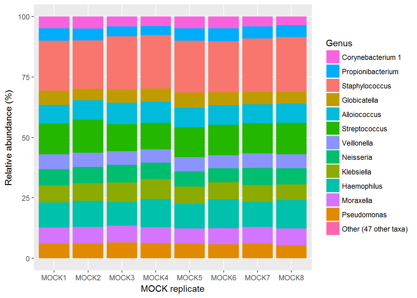

Again, the table may be more useful:

taxa	MOCK31	MOCK32	MOCK33	MOCK34	MOCK35	MOCK36	MOCK37	MOCK38
Corynebacterium 1	4.831868	5.029025	4.0849733	3.940035	4.804647	4.890366	4.158366	3.613126
Propionibacterium	5.151673	4.881288	4.0923028	3.734198	5.193078	5.369925	4.973969	4.809393
Staphylococcus	20.668246	19.984779	21.9384078	22.121677	21.377706	21.056727	22.001475	22.804263
Globicatella	5.915727	4.809658	5.5985146	5.522652	6.332126	5.446315	5.219420	4.796126
Alloiococcus	7.712791	8.001671	8.7648575	8.734489	8.046822	7.974254	7.832433	7.991332
Streptococcus	12.713259	13.644029	11.1554953	10.827815	12.393050	12.568963	12.354022	13.017424
Veillonella	6.130491	5.949769	5.7011275	5.555663	5.947194	5.500071	6.092259	5.762427
Neisseria	6.657032	6.598917	7.3014012	6.833408	6.218396	5.695289	7.058655	6.589422
Klebsiella	7.140085	7.301786	8.1699466	8.217954	7.019754	7.109916	7.025635	6.472227
Haemophilus	10.387647	10.796735	9.7103627	11.600676	10.267178	11.970576	10.354088	11.834424
Moraxella	6.675766	6.985420	6.9214889	6.579024	6.283135	6.576602	6.824211	6.921104
Pseudomonas	6.006717	6.003492	6.5159233	6.309105	6.106416	5.826850	6.088957	5.337874
Other (47 other taxa)	0.008708	0.013420	0.0451954	0.023290	0.010500	0.014140	0.016500	0.050847

It looks like the MOCK replicates across the four sequencing runs (two each) are very consistent, and represent very closely the expected theoretical composition. However, I wanted to test this: so I used a QIIME script to correlate the expected MOCK composition to these sequenced MOCKs.

The mock community contained 16 species at equal concentrations, so each one should make up 6.25% of the sample. I included some species from the same genus, so those ones should add up accordingly.

I made a file that contained all of the taxonomy strings representing the genera I included in the positive control, and the proportion that they should be present in (expected_mock3.txt). This was my “expected” mock community, which I correlated against my observed mock communities in QIIME:

compare_taxa_summaries.py -i taxa_summaries/mock3_only/final_otu_table_mock3_L6.txt,taxa_summaries/mock3_only/expected_mock3.txt -o mock3_compare -m expected

The output from this script includes a Pearson correlation coefficient with p-value and confidence interval, showing me that they were extremely similar.

Negative sequencing controls

I also needed to look at the taxa that were present in the negative controls. Firstly, it was important to check that the major contaminant taxa there were not abundant in the samples, and secondly I wanted to test whether the contamination was consistent (indicating reagent or workspace contamination). Reagents and workspaces are probably always contaminated no matter what you do, so I wanted to know if there were any consistent contaminants that I needed to look out for in the samples. My expectation was that if there was no strong contaminant signal, the contaminants were less likely to be consistent enough in the samples to interfere with results.

I did not produce a plot for this one, but I looked at the most abundant genera and created a table:

# QIIME taxa summary of negative controls with taxonomy changed to just genus name
negdata <- read.table("data/neg_only_genus_summary.txt", header = TRUE, sep = "\t")

# Collapse anything with a total of less than 1.0% into "Other" 
negdata$taxa <- ifelse(rowSums(negdata[,2:17]/16) < 0.01, "Other", as.character(negdata$taxa))
other <- negdata[which(negdata$taxa == "Other"),]
other <- colSums(other[2:17])
negdata <- negdata[-which(negdata$taxa == "Other"),]
other <- append(other, "Other (45 other taxa)")
names(other)[17] <- "taxa"
other <- other[c(17,1:16)]
negdata <- rbind(negdata,as.data.frame(t(other)))

# Make all numeric
for (i in 2:length(negdata)) {
  negdata[,i] <- as.numeric(negdata[,i])
}

# Make it a percentage
negdata[2:17] <- negdata[2:17] * 100

kable(negdata, row.names = FALSE)

taxa	Negex13	Negex1	NegPCR1	NegPCR2	Negex19	Negex32	NegPCR3	NegPCR4	Negex46	Negex55	NegPCR5	NegPCR6	Negex11	Negex64	NegPCR7	NegPCR8
Corynebacterium 1	0.0542594	0.3853565	0.0383436	0.0000000	7.294833	0.2433090	0.6835789	3.2915361	3.9800995	1.3592233	0.1203369	0.2580645	0.0000000	0.000000	0.1703578	0.0000000
Propionibacterium	1.5735214	0.1926782	0.0000000	0.0000000	2.127660	0.0000000	0.0151906	0.0000000	13.9303483	0.7766990	0.0000000	0.1290323	0.0000000	0.000000	0.1703578	0.0000000
Bacillus	29.4628323	28.9017341	0.0383436	12.6748971	16.818642	6.9343066	0.0000000	0.0000000	0.0000000	4.0776699	0.8423586	19.6129032	0.0000000	12.903226	0.0000000	0.0000000
Geobacillus	4.0694520	13.8728324	0.0000000	0.0000000	2.938197	0.0000000	0.0000000	0.0000000	0.0000000	1.9417476	0.0000000	0.0000000	0.0000000	1.075269	0.0000000	0.0000000
Lysinibacillus	0.0000000	0.0000000	0.0000000	0.0000000	9.017224	0.0000000	0.0000000	12.6175549	44.7761194	4.0776699	12.7557160	0.0000000	26.5017668	0.000000	14.1396934	47.1571906
Staphylococcus	0.1627781	4.4315992	0.3834356	1.7283951	8.611955	0.0000000	3.2963694	1.1755486	8.9552239	0.5825243	1.2033694	0.6451613	3.1802120	15.053763	5.7921635	3.0100334
Alloiococcus	4.6120456	0.0000000	0.4984663	0.5761317	14.792300	53.6496350	2.3393590	60.8150470	7.4626866	17.2815534	1.9253911	6.5806452	18.0212014	20.430107	6.3032368	0.8361204
Rhizobium	5.5344547	5.0096339	20.3987730	10.2880658	2.836879	0.0000000	0.2886222	2.5078370	0.4975124	16.1165049	10.2286402	21.0322581	1.7667845	0.000000	5.7921635	1.8394649
Delftia	44.8724905	27.5529865	73.3895706	72.1810700	2.026343	1.2165450	0.0000000	0.1567398	0.0000000	12.2330097	29.3622142	0.0000000	27.5618375	0.000000	18.9097104	10.0334448
Escherichia-Shigella	0.0000000	0.0000000	0.0000000	0.0000000	0.000000	0.0000000	87.5740544	0.0000000	0.0000000	0.0000000	0.0000000	0.0000000	0.0000000	0.000000	0.0000000	0.0000000
Haemophilus	2.0075963	9.4412331	1.5720859	0.9053498	8.004053	3.7712895	0.0759532	0.3134796	3.9800995	0.9708738	19.0132371	1.1612903	0.0000000	15.053763	1.0221465	0.0000000
Acinetobacter	2.1703744	0.0000000	0.0000000	0.0000000	11.043566	0.8515815	0.0000000	0.0000000	0.0000000	0.0000000	6.1371841	0.0000000	0.0000000	0.000000	0.0000000	0.0000000
Moraxella	3.7438958	2.8901734	0.8052147	0.6584362	3.748734	17.3965937	1.4431110	2.1159875	2.4875622	3.8834951	0.9626955	3.8709677	0.3533569	12.903226	1.3628620	0.0000000
Pseudomonas	0.0000000	0.1926782	0.1533742	0.0000000	6.889564	2.4330900	3.6001823	14.0282132	11.4427861	32.6213592	16.6064982	41.8064516	18.0212014	7.526882	44.1226576	32.9431438
Other (45 other taxa)	1.7362997	7.1290944	2.7223927	0.9876542	3.850051	13.5036495	0.6835788	2.9780564	2.4875622	4.0776701	0.8423585	4.9032260	4.5936396	15.053763	2.2146510	4.1806021

The most abundant contaminants are OTU41, OTU58, OTU1, OTU64, which would be most likely to appear in the samples. OTU1 is Alloiococcus is abundant in some of the negative controls, but we found lots of it in the middle ear and ear canal samples, and hardly at all in the nasopharynx. This indicates to me that it is likely to have ended up in the negative controls as a result of cross-contamination from samples rather than the other way around.

I checked the abundance of the other three across the samples themselves:

# OTU table contains only clinical samples above 1499 reads
otu.table <- read.table("data/final_otu_table_samples.txt", sep = "\t", header = T)

# Create abundance table
rownames(otu.table) <- otu.table$taxa
otu.table$taxa <- NULL
otu.total <- colSums(otu.table)
otu.abund <- otu.table
for (i in 1:length(otu.abund)) {
otu.abund[, i] <- otu.abund[, i]/otu.total[i] *
100
}

# Mean abundance across samples
sample.otu.mean <- rowSums(otu.abund)/length(otu.abund)
sample.otu.mean[grep("OTU41", names(sample.otu.mean))]

##      OTU41 
## 0.09111572

sample.otu.mean[grep("OTU58", names(sample.otu.mean))]

##      OTU58 
## 0.05113759

sample.otu.mean[grep("OTU64", names(sample.otu.mean))]

##      OTU64 
## 0.01275775

# Median abundance
sample.otu.medians <- apply(otu.abund, 1, median)
sample.otu.medians[grep("OTU41", names(sample.otu.medians))]

##       OTU41 
## 0.002617184

sample.otu.medians[grep("OTU58", names(sample.otu.medians))]

##      OTU58 
## 0.00299904

sample.otu.medians[grep("OTU64", names(sample.otu.medians))]

## OTU64 
##     0

These OTUs are very low in the clinical samples.

Having confirmed this, I then wanted to see whether the negative controls were similar to each other.

For this, I correlated the taxa summaries again but this time in “paired” rather than “expected” mode. I made three comparisons: 1. Negex-NegPCR pairs from the same plate 2. Negex-Negex pairs from the same run 3. NegPCR-NegPCR pairs from the same run

To set up the files for compare_taxa_summaries.py I first subsetted the OTU table to contain only the samples I wanted to compare. This was done twice for each comparison (e.g. for comparison 1, all of the Negex samples were in one OTU table and the NegPCR in another).

# Subset OTU table by sample names designated in text file
filter_samples_from_otu_table.py -i ../final_otu_table_all.biom -o pair1_1.biom
--sample_id_fp pair1_1.txt

I repeated this for each comparison (1_2, 2_1, 2_2 and so on). The purpose being, I can then summarise each OTU table giving me two taxonomy summaries to compare per comparison:

# Genus-level taxonomy summaries - repeated for each table
summarize_taxa.py -i pair1_1.biom --suppress_biom_table_output -L 6

Each comparison now has two taxonomy summary files to compare; lastly, I needed to indicate to the script which samples go together as pairs. I made files like this:

Negex1  Ex1
Negex19 Ex2
Negex13 Ex1
Negex32 Ex2

to show that Negex1 and Negex13 go together, Negex19 and Negex32, etc. This gives each pair of samples a “new name” and is passed with the -s flag in the script.

Finally, to do the comparisons (specifying paired mode with -m):

compare_taxa_summaries.py -i pair1_1_L6.txt,pair1_2_L6.txt -o pair1 -m paired -s
pair1_map.txt
compare_taxa_summaries.py -i pair2_1_L6.txt,pair2_2_L6.txt -o pair2 -m paired -s
pair2_map.txt
compare_taxa_summaries.py -i pair3_1_L6.txt,pair3_2_L6.txt -o pair3 -m paired -s
pair3_map.txt

From these correlation coefficients, I saw that there was a correlation between the pairs but it was only moderate (~0.5-0.6).