Differential abundance with metagenomeSeq’s fitZIG

Having explored the beta diversity with the PCoA plots, it was clear that the nasopharyngeal microbiome was different between the cases and controls, and within the cases the nasopharynx was distinct from the middle ear.

I wanted to investigate what makes these microbiomes distinct: which bacteria are differentially abundant between groups? This was also required to answer the research questions we had:

Do the controls have commensal bacteria that might be protective against ear infections?
Do some of the cases have novel otopathogens (bacteria that cause ear infections)?
Are the middle ear rinse samples more diverse than the middle ear fluid samples because they contain bacteria from biofilm which are not abundant in planktonic form?
Are the middle ear fluid samples contaminated by the bacteria in the ear canal?

I used the bioconductor package metagenomeSeq, which is designed for identifying differentially abundant OTUs in microbiome data. This package has a function called fitZIG, which builds a model (that can account for other variables) to determine differentially abundant OTUs, the adjusted p-value for the difference, and the log fold change between the groups compared. For the most part, I followed the vignette

I created five major models:

Case NPS/control NPS
Case MEF/case MER (paired analysis; same ear within the same child)
Case MEF/case NPS (paired analysis as above)
Case MER/case NPS (paired analysis as above)
Case ECS/case MEF (paired analysis as above)

The PCoA/Procrustes analysis showed that the fluid and rinse sample types weren’t too similar. Because of this, I compared both the fluid and the rinse to the nasopharynx.

The left and right ears were also not too similar, but with these paired analyses I had to select only one ear per child. I addressed this issue by selecting one ear per child at random (Set 1), and then repeating the analysis but with the opposite ear (Set 2). Any OTUs that were not in agreement between the two sets I considered false positives.

Here are the major steps for the differential abundance analysis. Be aware that TONS of code follows as I have documented its use for each model including the Set 1/Set 2 validation.

Creating the metagenomeSeq object

metagenomeSeq requires information on the samples in the form of a metagenomeSeq object. Firstly, to determine the samples that were included in the models:

For model 1, I simply subsetted the OTU table to only NPS samples above 1499 reads. For models 2-4, I had to select one sample per child at random (not for model 5 as we only took one ear canal swab per child). I won’t burden this page with data wrangling code, so here are the major steps I took to get to that point:

Took a list of all case samples
Subsetted this list to the appropriate sample types depending on the model
Removed samples that had no pair for analysis
Where both left and right ears were available, I selected one at random with sample(c("left","right"), 1) until I had one pair of samples per child
Subsetted the OTU table to these chosen samples
Read this in to metagenomeSeq as below

I also created an OTU table with the opposite ear selected instead. I kept those pairs of samples that had no alternative (e.g. NPS with left fluid, but no right fluid available for that child) but swapped out those where two pairs were available (e.g. NPS with left fluid became NPS with right fluid). The purpose of this was to identify the differentially abundant OTUs on which the two models were in agreement.

A metagenomeSeq object requires three things: the OTU count table, the taxonomy, and any relevant phenotypic data.

I begin by reading in the OTU table:

library(metagenomeSeq)
## Read in the OTU table (raw) with no taxonomy in it

# Model 1
nps <- loadMeta("data/nps_otus.txt", sep = "\t")

# Model 2
FR <- loadMeta("data/FR_otus.txt", sep = "\t")

# Model 2 opposite pairs
FR2 <- loadMeta("data/FR2_otus.txt", sep = "\t")

# Model 3
FNPS <- loadMeta("data/FNPS_otus.txt", sep = "\t")

# Model 3 opposite pairs
FNPS2 <- loadMeta("data/FNPS2_otus.txt", sep = "\t")

# Model 4
RNPS <- loadMeta("data/RNPS_otus.txt", sep = "\t")

# Model 4 opposite pairs
RNPS2 <- loadMeta("data/RNPS2_otus.txt", sep = "\t")

# Model 5
EF <- loadMeta("data/EF_otus.txt", sep = "\t")

# To check it read in the right number of samples and OTUs
# e.g.
dim(nps$counts)

## [1] 123 188

The taxonomy was the same for all models as all tables contained the full 123 OTUs. The OTUs are in the same order in the OTU tables and in this taxonomy file. I have modified the taxonomy so there is one column for the OTU ID, then subsequent columns for Kingdom/Phylum/Class etc.

Note that I didn’t actually notice the taxonomy being used in any of the functions I used; so I can’t guarantee this is actually formatted correctly

# Read in the taxonomy strings separated by taxonomy levels
taxa <- read.delim("data/taxonomy_raw.txt", stringsAsFactors = FALSE, sep = "\t")

And finally, the phenotypic information about the samples.

For model 1, I needed information on the antibiotic usage, gender and length of breastfeeding as these were confounding factors that I wanted to take into account. For the other models, I am comparing pairs within the same child, so these are not needed and I only included sample type.

## Read in the relevant sample metadata including sample type (group)

# Model 1
meta <- loadPhenoData("data/nps_metadata.txt", sep = "\t", tran = TRUE)

# Model 2
FR.meta <- loadPhenoData("data/FR_metadata_sorted.txt", sep = "\t", tran = TRUE)

# Model 2 opposite pairs
FR2.meta <- loadPhenoData("data/FR2_metadata_sorted.txt", sep = "\t", tran = TRUE)

# Model 3
FNPS.meta <- loadPhenoData("data/FNPS_metadata_sorted.txt", sep = "\t", tran = TRUE)

# Model 3 opposite pairs
FNPS2.meta <- loadPhenoData("data/FNPS2_metadata_sorted.txt", sep = "\t", tran = TRUE)

# Model 4
RNPS.meta <- loadPhenoData("data/RNPS_metadata_sorted.txt", sep = "\t", tran = TRUE)

# Model 4 opposite pairs
RNPS2.meta <- loadPhenoData("data/RNPS2_metadata_sorted.txt", sep = "\t", tran = TRUE)

# Model 5
EF.meta <- loadPhenoData("data/EF_metadata_sorted.txt", sep = "\t", tran = TRUE)

## Make sure samples in OTU table and in metdata are in the same order

# Model 1
ord <- match(colnames(nps$counts), rownames(meta))
meta <- meta[ord,]

# Model 2 
ord <- match(rownames(FR.meta),colnames(FR$counts))
FR$counts <- FR$counts[,ord]

# Model 2 opposite pairs
ord <- match(rownames(FR2.meta),colnames(FR2$counts))
FR2$counts <- FR2$counts[,ord]

# Model 3
ord <- match(rownames(FNPS.meta),colnames(FNPS$counts))
FNPS$counts <- FNPS$counts[,ord]

# Model 3 opposite pairs
ord <- match(rownames(FNPS2.meta),colnames(FNPS2$counts))
FNPS2$counts <- FNPS2$counts[,ord]

# Model 4
ord <- match(rownames(RNPS.meta),colnames(RNPS$counts))
RNPS$counts <- RNPS$counts[,ord]

# Model 4 opposite pairs
ord <- match(rownames(RNPS2.meta),colnames(RNPS2$counts))
RNPS2$counts <- RNPS2$counts[,ord]

# Model 5
ord <- match(rownames(EF.meta),colnames(EF$counts))
EF$counts <- EF$counts[,ord]

Now that all of this information has been read in, I convert it all into one object per model for metagenomeSeq to work with.

## Create one MRexperiment object per model

# Model 1
phenotypeData <- AnnotatedDataFrame(meta)
OTUdata <- AnnotatedDataFrame(taxa)
# Row names need to become OTU IDs so it matches the rownames in count table; this gets used for all models
row.names(OTUdata) <- taxa$taxa
OTUdata

## An object of class 'AnnotatedDataFrame'
##   rowNames: OTU5 OTU2 ... OTU52 (123 total)
##   varLabels: taxa Kingdom ... X (8 total)
##   varMetadata: labelDescription

# Create model
npsdata <- newMRexperiment(nps$counts, phenoData = phenotypeData, featureData = OTUdata)
# Removed samples with NA for metadata (only a few): I did get an error when they were left in, not certain if this needs to be done
keep1 <- !is.na(npsdata$ab_pastmonth)
npsdata <- npsdata[,keep1]
keep2 <- !is.na(npsdata$breastfed_cease_months)
npsdata <- npsdata[,keep2]

# Model 2
FR.phenotypeData <- AnnotatedDataFrame(FR.meta)
# Make object
FRdata <- newMRexperiment(FR$counts, phenoData = FR.phenotypeData, featureData = OTUdata)

# Model 2 opposite pairs
FR2.phenotypeData <- AnnotatedDataFrame(FR2.meta)
# Make object
FR2data <- newMRexperiment(FR2$counts, phenoData = FR2.phenotypeData, featureData = OTUdata)

# Model 3
FNPS.phenotypeData <- AnnotatedDataFrame(FNPS.meta)
# Make object
FNPSdata <- newMRexperiment(FNPS$counts, phenoData = FNPS.phenotypeData, featureData = OTUdata)

# Model 3 opposite pairs
FNPS2.phenotypeData <- AnnotatedDataFrame(FNPS2.meta)
FNPS2data <- newMRexperiment(FNPS2$counts, phenoData = FNPS2.phenotypeData, featureData = OTUdata)

# Model 4
RNPS.phenotypeData <- AnnotatedDataFrame(RNPS.meta)
# Make object
RNPSdata <- newMRexperiment(RNPS$counts, phenoData = RNPS.phenotypeData, featureData = OTUdata)

# Model 4 opposite pairs
RNPS2.phenotypeData <- AnnotatedDataFrame(RNPS2.meta)
RNPS2data <- newMRexperiment(RNPS2$counts, phenoData = RNPS2.phenotypeData, featureData = OTUdata)

# Model 5
EF.phenotypeData <- AnnotatedDataFrame(EF.meta)
# Make object
EFdata <- newMRexperiment(EF$counts, phenoData = EF.phenotypeData, featureData = OTUdata)

Normalising the data

I now have one MRexperiment object per model. The next step is to normalise the data to account for differences due to uneven sequencing depth. Rather than rarefying, metagenomeSeq uses Cumulative Sum Scaling (CSS) normalisation which was developed for microbiome data. This is the method that I used to normalise the data when I plotted and statistically compared alpha diversity.

There are a couple of steps here; firstly, to try and reduce false positives I’ve removed low abundance OTUs. I’ve defined this as OTUs that aren’t present in at least 25% of samples; so this number is different for each model.

## Removing low-abundance OTUs

# Model 1 (takes down to 82 OTUs).
npsdata.trim <- filterData(npsdata, present = 46)

# Model 2 (down to 50 OTUs)
FRdata.trim <- filterData(FRdata, present = 25)

# Model 2 opposite pairs (down to 50 OTUs) 
FR2data.trim <- filterData(FR2data, present = 25)

# Model 3 (down to 82 OTUs)
FNPSdata.trim <- filterData(FNPSdata, present = 37)

# Model 3 opposite pairs (down to 81 OTUs)
FNPS2data.trim <- filterData(FNPS2data, present = 37)

# Model 4 (down to 81 OTUs)
RNPSdata.trim <- filterData(RNPSdata, present = 27)

# Model 4 opposite pairs (down to 80 OTUs)
RNPS2data.trim <- filterData(RNPS2data, present = 27)

# Model 5 (down to 50 OTUs)
EFdata.trim <- filterData(EFdata, present = 16)

Then I normalise the table. I also exported a table of normalised and logged counts for use later on.

## Normalising the OTU counts
# Model 1
p <- cumNormStatFast(npsdata.trim)
npsdata.trim <- cumNorm(npsdata.trim, p = p)
# Export count matrix
npsnorm <- MRcounts(npsdata.trim, norm = TRUE, log = TRUE)
#write.table(npsnorm, "normalised_logged_184samples.txt", sep = "\t")

# Model 2
p <- cumNormStatFast(FRdata.trim)
FRdata.trim <- cumNorm(FRdata.trim, p = p)
# Export count matrix
FRnorm <- MRcounts(FRdata.trim, norm = TRUE, log = TRUE)
#write.table(FRnorm, "FRdata_normalised_logged.txt", sep = "\t")

# Model 2 opposite pairs
p <- cumNormStatFast(FR2data.trim)
FR2data.trim <- cumNorm(FR2data.trim, p = p)
# Export count matrix
FR2norm <- MRcounts(FR2data.trim, norm = TRUE, log = TRUE)
#write.table(FR2norm, "FR2data_normalised_logged.txt", sep = "\t")

# Model 3
p <- cumNormStatFast(FNPSdata.trim)
FNPSdata.trim <- cumNorm(FNPSdata.trim, p = p)
# Export count matrix
FNPSnorm <- MRcounts(FNPSdata.trim, norm = TRUE, log = TRUE)
#write.table(FNPSnorm, "FNPSdata_normalised_logged.txt", sep = "\t")

# Model 3 opposite pairs
p <- cumNormStatFast(FNPS2data.trim)
FNPS2data.trim <- cumNorm(FNPS2data.trim, p = p)
# Export count matrix
FNPS2norm <- MRcounts(FNPS2data.trim, norm = TRUE, log = TRUE)
#write.table(FNPS2norm, "FNPS2data_normalised_logged.txt", sep = "\t")

# Model 4 
p <- cumNormStatFast(RNPSdata.trim)
RNPSdata.trim <- cumNorm(RNPSdata.trim, p = p)
# Export count matrix
RNPSnorm <- MRcounts(RNPSdata.trim, norm = TRUE, log = TRUE)
#write.table(RNPSnorm, "RNPSdata_normalised_logged.txt", sep = "\t")

# Model 4 opposite pairs
p <- cumNormStatFast(RNPS2data.trim)
RNPS2data.trim <- cumNorm(RNPS2data.trim, p = p)
# Export count matrix
RNPS2norm <- MRcounts(RNPS2data.trim, norm = TRUE, log = TRUE)
#write.table(RNPS2norm, "RNPS2data_normalised_logged.txt", sep = "\t")

# Model 5
p <- cumNormStatFast(EFdata.trim)
EFdata.trim <- cumNorm(EFdata.trim, p = p)
# Export count matrix
EFnorm <- MRcounts(EFdata.trim, norm = TRUE, log = TRUE)
#write.table(EFnorm, "EFdata_normalised_logged.txt", sep = "\t")

fitZIG models

The CSS normalised data is now ready for use. I used the fitZIG function to build a model because it has the ability to include other variables as covariates, which is important for the comparison between cases and controls.

I made five major models, but remember that for models 2-4 I ran it again with the set of opposite-ear pairs (which I call Set 2) as a form of validation. For all models I checked the exported list of coefficients to make sure that no significantly different OTUs had been left off the list (top 40 OTUs was usually enough to show them all). To get this code, I followed the metagenomeSeq vignette.

Model 1 (case/control NPS including other covariates)

# Define the metadata categories we want to use:
status <- pData(npsdata.trim)$group
gender <- pData(npsdata.trim)$gender
antibiotic <- pData(npsdata.trim)$ab_pastmonth
bfed <- pData(npsdata.trim)$breastfed_cease_months

# Define the normalisation factor
norm.factor <- normFactors(npsdata.trim)
norm.factor <- log2(norm.factor/median(norm.factor) + 1)

# Create the model
mod <- model.matrix(~ status + gender + antibiotic + bfed + norm.factor)
settings <- zigControl(maxit = 10, verbose = TRUE)
fit <- fitZig(obj = npsdata.trim, mod = mod, useCSSoffset = FALSE, control = settings)

## it= 0, nll=303.66, log10(eps+1)=Inf, stillActive=83
## it= 1, nll=339.99, log10(eps+1)=0.00, stillActive=1
## it= 2, nll=340.77, log10(eps+1)=0.00, stillActive=0

# Generate table of log fold change coefficients for each OTU, sorting by adjusted p-value
coefs <- MRcoefs(fit, coef = 2, group = 3, number = 40)

# Export the coefficients and adjusted p-values
#write.table(coefs, "fit_results.txt", sep = "\t")

The results from this model have been adjusted for gender, antibiotic use and length of breastfeeding; all of which were categorical variables.

The other models are more straightforward and compare pairs of samples from the same case child.

Model 2 (MEF/MER)

# Define the metadata categories
FR.type <- pData(FRdata.trim)$type
FR.ID <- pData(FRdata.trim)$ID

# Define the normalisation factor
FR.norm.factor <- normFactors(FRdata.trim)
FR.norm.factor <- log2(FR.norm.factor/median(FR.norm.factor) + 1)

# Create the model
FR.mod <- model.matrix(~ FR.type + FR.ID + FR.norm.factor)
settings <- zigControl(maxit = 10, verbose = TRUE)
FR.fit <- fitZig(obj = FRdata.trim, mod = FR.mod, useCSSoffset = FALSE, control = settings)

## it= 0, nll=143.06, log10(eps+1)=Inf, stillActive=50
## it= 1, nll=152.73, log10(eps+1)=0.01, stillActive=2
## it= 2, nll=152.91, log10(eps+1)=0.00, stillActive=0

# Get table of coefficients
FR.coefs <- MRcoefs(FR.fit, coef = 2, group = 3, number = 40)
#write.table(FR.coefs, "FR_fit_results.txt", sep = "\t")

# Running again with Set 2 samples (opposite ears)

# Define metadata categories
FR2.type <- pData(FR2data.trim)$type
FR2.ID <- pData(FR2data.trim)$ID

# Define normalisation factor
FR2.norm.factor <- normFactors(FR2data.trim)
FR2.norm.factor <- log2(FR2.norm.factor/median(FR2.norm.factor) + 1)

# Create model
FR2.mod <- model.matrix(~ FR2.type + FR2.ID + FR2.norm.factor)
settings <- zigControl(maxit = 10, verbose = TRUE)
FR2.fit <- fitZig(obj = FR2data.trim, mod = FR2.mod, useCSSoffset = FALSE, control = settings)

## it= 0, nll=143.73, log10(eps+1)=Inf, stillActive=50
## it= 1, nll=153.43, log10(eps+1)=0.00, stillActive=1
## it= 2, nll=153.35, log10(eps+1)=0.00, stillActive=0

# Get coefficients and export
FR2.coefs <- MRcoefs(FR2.fit, coef = 2, group = 3, number = 40)
#write.table(FR2.coefs, "FR2_fit_results.txt", sep = "\t")

Model 3 (MEF/NPS)

# Define the metadata categories
FNPS.type <- pData(FNPSdata.trim)$type
FNPS.ID <- pData(FNPSdata.trim)$ID

# Define the normalisation factor
FNPS.norm.factor <- normFactors(FNPSdata.trim)
FNPS.norm.factor <- log2(FNPS.norm.factor/median(FNPS.norm.factor) + 1)

# Create the model
# dfMethod = "default" for big designs to remove NaN warnings
FNPS.mod <- model.matrix(~ FNPS.type + FNPS.ID + FNPS.norm.factor)
settings <- zigControl(maxit = 10, verbose = TRUE, dfMethod = "default")
FNPS.fit <- fitZig(obj = FNPSdata.trim, mod = FNPS.mod, useCSSoffset = FALSE, control = settings)

## it= 0, nll=207.56, log10(eps+1)=Inf, stillActive=82
## it= 1, nll=217.65, log10(eps+1)=0.04, stillActive=9
## it= 2, nll=217.28, log10(eps+1)=0.01, stillActive=5
## it= 3, nll=216.81, log10(eps+1)=0.01, stillActive=2
## it= 4, nll=216.04, log10(eps+1)=0.01, stillActive=1
## it= 5, nll=215.43, log10(eps+1)=0.00, stillActive=0

# Get table of coefficients
FNPS.coefs <- MRcoefs(FNPS.fit, coef = 2, group = 3, number = 50)
#write.table(FNPS.coefs, "FNPS_fit_results.txt", sep = "\t")

# Run again with Set 2 samples

# Define metadata
FNPS2.type <- pData(FNPS2data.trim)$type
FNPS2.ID <- pData(FNPS2data.trim)$ID

# Define normalisation factor
FNPS2.norm.factor <- normFactors(FNPS2data.trim)
FNPS2.norm.factor <- log2(FNPS2.norm.factor/median(FNPS2.norm.factor) + 1)

# Create model
FNPS2.mod <- model.matrix(~ FNPS2.type + FNPS2.ID + FNPS2.norm.factor)
settings <- zigControl(maxit = 10, verbose = TRUE, dfMethod = "default")
FNPS2.fit <- fitZig(obj = FNPS2data.trim, mod = FNPS2.mod, useCSSoffset = FALSE, control = settings)

## it= 0, nll=208.91, log10(eps+1)=Inf, stillActive=81
## it= 1, nll=219.90, log10(eps+1)=0.02, stillActive=8
## it= 2, nll=219.51, log10(eps+1)=0.01, stillActive=3
## it= 3, nll=218.80, log10(eps+1)=0.00, stillActive=1
## it= 4, nll=217.99, log10(eps+1)=0.02, stillActive=1
## it= 5, nll=217.60, log10(eps+1)=0.00, stillActive=0

# Get coefficients and export
FNPS2.coefs <- MRcoefs(FNPS2.fit, coef = 2, group = 3, number = 50)
#write.table(FNPS2.coefs, "FNPS2_fit_results.txt", sep = "\t")

Model 4 (MER/NPS)

# Define the metadata categories we want to use:
RNPS.type <- pData(RNPSdata.trim)$type
RNPS.ID <- pData(RNPSdata.trim)$ID

# Define the normalisation factor
RNPS.norm.factor <- normFactors(RNPSdata.trim)
RNPS.norm.factor <- log2(RNPS.norm.factor/median(RNPS.norm.factor) + 1)

# Create the model
RNPS.mod <- model.matrix(~ RNPS.type + RNPS.ID + RNPS.norm.factor)
settings <- zigControl(maxit = 10, verbose = TRUE)
RNPS.fit <- fitZig(obj = RNPSdata.trim, mod = RNPS.mod, useCSSoffset = FALSE, control = settings)

## it= 0, nll=154.49, log10(eps+1)=Inf, stillActive=81
## it= 1, nll=165.97, log10(eps+1)=0.03, stillActive=5
## it= 2, nll=165.58, log10(eps+1)=0.01, stillActive=3
## it= 3, nll=165.28, log10(eps+1)=0.01, stillActive=1
## it= 4, nll=164.92, log10(eps+1)=0.00, stillActive=0

# Get table of coefficients and export
RNPS.coefs <- MRcoefs(RNPS.fit, coef = 2, group = 3, number = 40)
#write.table(RNPS.coefs, "RNPS_fit_results.txt", sep = "\t")

# Run again with Set 2 samples

# Define metadata 
RNPS2.type <- pData(RNPS2data.trim)$type
RNPS2.ID <- pData(RNPS2data.trim)$ID

# Define normalisation factor
RNPS2.norm.factor <- normFactors(RNPS2data.trim)
RNPS2.norm.factor <- log2(RNPS2.norm.factor/median(RNPS2.norm.factor) + 1)

# Create the model
RNPS2.mod <- model.matrix(~ RNPS2.type + RNPS2.ID + RNPS2.norm.factor)
settings <- zigControl(maxit = 10, verbose = TRUE, dfMethod = "default")
RNPS2.fit <- fitZig(obj = RNPS2data.trim, mod = RNPS2.mod, useCSSoffset = FALSE, control = settings)

## it= 0, nll=153.05, log10(eps+1)=Inf, stillActive=80
## it= 1, nll=162.27, log10(eps+1)=0.01, stillActive=8
## it= 2, nll=161.56, log10(eps+1)=0.02, stillActive=5
## it= 3, nll=160.96, log10(eps+1)=0.01, stillActive=1
## it= 4, nll=160.20, log10(eps+1)=0.01, stillActive=1
## it= 5, nll=159.65, log10(eps+1)=0.01, stillActive=1
## it= 6, nll=159.50, log10(eps+1)=0.00, stillActive=0

# Get coefficients and export
RNPS2.coefs <- MRcoefs(RNPS2.fit, coef = 2, group = 3, number = 40)
#write.table(RNPS2.coefs, "RNPS2_fit_results.txt", sep = "\t")

Model 5 (ECS/MEF)

# Define the metadata categories we want to use:
EF.type <- pData(EFdata.trim)$type
EF.ID <- pData(EFdata.trim)$ID

# Define the normalisation factor
EF.norm.factor <- normFactors(EFdata.trim)
EF.norm.factor <- log2(EF.norm.factor/median(EF.norm.factor) + 1)

# Create the model
EF.mod <- model.matrix(~ EF.type + EF.ID + EF.norm.factor)
settings <- zigControl(maxit = 10, verbose = TRUE)
EF.fit <- fitZig(obj = EFdata.trim, mod = EF.mod, useCSSoffset = FALSE, control = settings)

## it= 0, nll=93.90, log10(eps+1)=Inf, stillActive=50
## it= 1, nll=102.17, log10(eps+1)=0.02, stillActive=2
## it= 2, nll=102.10, log10(eps+1)=0.02, stillActive=1
## it= 3, nll=102.00, log10(eps+1)=0.00, stillActive=0

# Get table of coefficients and export
EF.coefs <- MRcoefs(EF.fit, coef = 2, group = 3, number = 40)
#write.table(EF.coefs, "EF_fit_results.txt", sep = "\t")

Identifying the important OTUs

In the XX_fit_results.txt files I now have a list of all of the OTUs that are significantly differentially abundant between the two groups I compared.

I need to filter through these to determine which OTUs are probably false positives to leave me with the OTUs that are likely to be of interest. For the models where I validated with the opposite ear, this involves comparing the significant OTUs from those two models and retaining only those that appeared in both. For all models, I also defined a threshold of abundance below which I considered those OTUs to be contaminants/not real. The threshold for the OTUs from each model was 0.35% mean or median abundance in at least one group; I chose this threshold as it removes the major negative control genus that came up as differentially abundant (Delftia) but retains a genus that I would expect to be found in the upper respiratory tract (Veillonella). This came from the MEF/NPS model.

Model 1: case/control NPS

Removed OTUs below threshold

# Get the list of OTUs with coefficients and p-values from fitZIG model
cc.sig.otus <- read.table("data/fit_results.txt", header = T, sep = "\t")

# Cut out those with an adjusted p-value of > 0.05
cc.sig.otus <- cc.sig.otus[-which(cc.sig.otus$adjPvalues >= 0.055),]
names(cc.sig.otus) <- c("OTU", "effectsize", "Pvalue", "adjPvalue")

# Read in the matrix of CSS normalised and logged counts
cc.normal.table <- read.table("data/normalised_logged_184samples.txt", header = T, sep = "\t", check.names = F)

# Subset this table to the significant OTUs and remove unnecessary columns
cc.sig.table <- merge(cc.sig.otus, cc.normal.table)
cc.sig.table$effectsize <- NULL
cc.sig.table$Pvalue <- NULL
cc.sig.table$adjPvalue <- NULL

# Transpose the table
rownames(cc.sig.table) <- cc.sig.table$OTU
cc.sig.table$OTU <- NULL
cc.sig.table <- t(cc.sig.table)

# Split into tables of cases and controls
cases.table <- subset(cc.sig.table,grepl("^M", rownames(cc.sig.table)))
controls.table <- subset(cc.sig.table,!grepl("^M", rownames(cc.sig.table)))

## Calculating relative abundance data at an OTU level

# Read in the raw OTU table containing all samples (doesn't contain taxonomy)
cc.full.table <- read.table("data/final_otu_table_samples.txt", sep = "\t", header = T, check.names = F)

# Subset OTU table to the samples in the model
cc.full.table <- cc.full.table[,c(1,which(names(cc.full.table) %in% rownames(cc.sig.table)))]
rownames(cc.full.table) <- cc.full.table$taxa
cc.full.table$taxa <- NULL

# Convert OTU table to relative abundance table by taking proportions of total
cc.abund.table <- sweep(cc.full.table,2,colSums(cc.full.table),`/`) * 100

# Subset the abundance table to the significantly differentially abundant OTUs and tranpose it
cc.abund.table <- t(cc.abund.table[which(rownames(cc.abund.table) %in% cc.sig.otus$OTU),])

# Split the abundance table into cases and controls
cases.abundance <- subset(cc.abund.table,grepl("^M", rownames(cc.abund.table)))
controls.abundance <- subset(cc.abund.table,!grepl("^M", rownames(cc.abund.table)))

# Put the tables of abundance and table of normalised values in the same order
# Cases
ord1 <- match(colnames(cases.abundance), colnames(cases.table))
cases.table <- cases.table[,ord1]
ord2 <- match(rownames(cases.abundance), rownames(cases.table))
cases.table <- cases.table[ord2,]
# Controls
ord3 <- match(colnames(controls.abundance), colnames(controls.table))
controls.table <- controls.table[,ord3]
ord4 <- match(rownames(controls.abundance), rownames(controls.table))
controls.table <- controls.table[ord4,]

## Selecting OTUs that have a mean or median of at least 0.35% 

# Work with data frames
cases.table <- as.data.frame(cases.table)
controls.table <- as.data.frame(controls.table)
cases.abundance <- as.data.frame(cases.abundance)
controls.abundance <- as.data.frame(controls.abundance)

# Select only OTUs above threshold
cc.threshold <- c()
for (i in 1:length(cases.table)) {
cc.threshold[i] <- ifelse(median(cases.abundance[,i]) > 0.35 | median(controls.abundance[,i]) > 0.35 | mean(cases.abundance[,i]) > 0.35 | mean(controls.abundance[,i]) > 0.35, names(cases.table[i]), NA)
}
cc.threshold <- cc.threshold[!is.na(cc.threshold)]
cc.threshold

##  [1] "OTU5"   "OTU6"   "OTU8"   "OTU10"  "OTU22"  "OTU13"  "OTU33" 
##  [8] "OTU24"  "OTU12"  "OTU35"  "OTU18"  "OTU20"  "OTU30"  "OTU434"
## [15] "OTU216" "OTU23"  "OTU25"

## Export table of mean and median values for all significant OTUs (including those below threshold)

# Determine mean and median values
cc.table <- cc.sig.otus$OTU
mean.ca.all <- c()
mean.co.all <- c()
median.ca.all <- c()
median.co.all <- c()

for (i in cc.table) {
  mean.ca.all[i] <- mean(cases.abundance[,i])
  median.ca.all[i] <- median(cases.abundance[,i])
  mean.co.all[i] <- mean(controls.abundance[,i])
  median.co.all[i] <- median(controls.abundance[,i])
}

# Combine into table
cc.table.full <- data.frame(mean.ca.all, median.ca.all, mean.co.all, median.co.all)

# Output table
#write.table(cc.table.full, "casecontrol_sig_otus_means_medians.txt", sep = "\t")

Model 2: MEF/MER

Removed OTUs that weren’t significant in both models (Set 1 and Set 2; the main model and the model with the opposite ears)
Removed OTUs below threshold

# Get the list of OTUs with coefficients and p-values from fitZIG models
# Set 1
FR.sig.otus <- read.table("data/FR_fit_results.txt", header = T, sep = "\t")
# Set 2
FR.sig2.otus <- read.table("data/FR2_fit_results.txt", header = T, sep = "\t")

# Cut out those with an adjusted p-value of > 0.05
# Set 1
FR.sig.otus <- FR.sig.otus[-which(FR.sig.otus$adjPvalues >= 0.055),]
names(FR.sig.otus) <- c("OTU", "effectsize", "Pvalue", "adjPvalue")
# Set 2
FR.sig2.otus <- FR.sig2.otus[-which(FR.sig2.otus$adjPvalues >= 0.055),]
names(FR.sig2.otus) <- c("OTU", "effectsize", "Pvalue", "adjPvalue")

# Read in the normalised and logged OTU table
# Set 1
FR.normal.table <- read.table("data/FRdata_normalised_logged.txt", header = T, sep = "\t")
# Set 2
FR.normal2.table <- read.table("data/FR2data_normalised_logged.txt", header = T, sep = "\t")

# Subset this OTU table to the significant OTUs and remove unnecessary columns
# Set 1
FR.sig.table <- merge(FR.sig.otus, FR.normal.table)
FR.sig.table$effectsize <- NULL
FR.sig.table$Pvalue <- NULL
FR.sig.table$adjPvalue <- NULL
# Set 2
FR.sig2.table <- merge(FR.sig2.otus, FR.normal2.table)
FR.sig2.table$effectsize <- NULL
FR.sig2.table$Pvalue <- NULL
FR.sig2.table$adjPvalue <- NULL

# Transpose the table
# Set 1
rownames(FR.sig.table) <- FR.sig.table$OTU
FR.sig.table$OTU <- NULL
FR.sig.table <- t(FR.sig.table)
# Set 2
rownames(FR.sig2.table) <- FR.sig2.table$OTU
FR.sig2.table$OTU <- NULL
FR.sig2.table <- t(FR.sig2.table)

# Split into tables of MEF and MER
# Set 1
fluids.table <- subset(FR.sig.table,grepl("F", rownames(FR.sig.table)))
rinses.table <- subset(FR.sig.table,!grepl("F", rownames(FR.sig.table)))
# Set 2
fluids2.table <- subset(FR.sig2.table,grepl("F", rownames(FR.sig2.table)))
rinses2.table <- subset(FR.sig2.table,!grepl("F", rownames(FR.sig2.table)))

## Calculate the relative abundance for threshold

# Read in full, raw OTU table of samples (no taxonomy)
FR.full.table <- read.table("data/final_otu_table_samples.txt", sep = "\t", header = T)

# Subset raw OTU table to the samples included in the models
# Set 1
FR.full1.table <- FR.full.table[,c(1,which(names(FR.full.table) %in% rownames(FR.sig.table)))]
rownames(FR.full1.table) <- FR.full.table$taxa
FR.full1.table$taxa <- NULL
# Set 2
FR.full2.table <- FR.full.table[,c(1,which(names(FR.full.table) %in% rownames(FR.sig2.table)))]
rownames(FR.full2.table) <- FR.full.table$taxa
FR.full2.table$taxa <- NULL

# Convert OTU table to relative abundance table by taking proportions of total
# Set 1
FR.abund1.table <- sweep(FR.full1.table,2,colSums(FR.full1.table),`/`) * 100
# Set 2
FR.abund2.table <- sweep(FR.full2.table,2,colSums(FR.full2.table), `/`) * 100

# Subset the abundance table to the significantly differentially abundant OTUs and tranpose it
# Set 1
FR.abund1.table <- t(FR.abund1.table[which(rownames(FR.abund1.table) %in% FR.sig.otus$OTU),])
# Set 2
FR.abund2.table <- t(FR.abund2.table[which(rownames(FR.abund2.table) %in% FR.sig2.otus$OTU),])

# Split abundance table into fluids and rinses
# Set 1
fluids.abundance <- subset(FR.abund1.table,grepl("F", rownames(FR.abund1.table)))
rinses.abundance <- subset(FR.abund1.table,!grepl("F", rownames(FR.abund1.table)))
# Set 2
fluids2.abundance <- subset(FR.abund2.table,grepl("F", rownames(FR.abund2.table)))
rinses2.abundance <- subset(FR.abund2.table,!grepl("F", rownames(FR.abund2.table)))

## Put the normalised counts table and the abundance table in the same order
# Fluids set 1
ord1 <- match(colnames(fluids.abundance), colnames(fluids.table))
fluids.table <- fluids.table[,ord1]
ord2 <- match(rownames(fluids.abundance), rownames(fluids.table))
fluids.table <- fluids.table[ord2,]
# Rinses set 1
ord3 <- match(colnames(rinses.abundance), colnames(rinses.table))
rinses.table <- rinses.table[,ord3]
ord4 <- match(rownames(rinses.abundance), rownames(rinses.table))
rinses.table <- rinses.table[ord4,]

# Fluids set 2
ord5 <- match(colnames(fluids2.abundance), colnames(fluids2.table))
fluids2.table <- fluids2.table[,ord5]
ord6 <- match(rownames(fluids2.abundance), rownames(fluids2.table))
fluids2.table <- fluids2.table[ord6,]
# Rinses set 2
ord7 <- match(colnames(rinses2.abundance), colnames(rinses2.table))
rinses2.table <- rinses2.table[,ord7]
ord8 <- match(rownames(rinses2.abundance), rownames(rinses2.table))
rinses2.table <- rinses2.table[ord8,]

## Selecting OTUs that have a mean or median of at least 0.35%

# Work with data frames (sorry for not knowing more efficient way)
fluids.table <- as.data.frame(fluids.table)
rinses.table <- as.data.frame(rinses.table)
fluids.abundance <- as.data.frame(fluids.abundance)
rinses.abundance <- as.data.frame(rinses.abundance)
fluids2.table <- as.data.frame(fluids2.table)
rinses2.table <- as.data.frame(rinses2.table)
fluids2.abundance <- as.data.frame(fluids2.abundance)
rinses2.abundance <- as.data.frame(rinses2.abundance)

# Select only OTUs above threshold
# Set 1
FR.threshold.1 <- c()
for (i in 1:length(fluids.table)) {
FR.threshold.1[i] <- ifelse(median(fluids.abundance[,i]) > 0.35 | median(rinses.abundance[,i]) > 0.35 | mean(fluids.abundance[,i]) > 0.35 | mean(rinses.abundance[,i]) > 0.35, names(fluids.table[i]), NA)
  }
FR.threshold.1 <- FR.threshold.1[!is.na(FR.threshold.1)]
FR.threshold.1

## [1] "OTU6"    "OTU1003" "OTU3"    "OTU1"    "OTU7"    "OTU269"  "OTU212"

# Set 2
FR.threshold.2 <- c()
for (i in 1:length(fluids2.table)) {
FR.threshold.2[i] <- ifelse(median(fluids2.abundance[,i]) > 0.35 | median(rinses2.abundance[,i]) > 0.35 | mean(fluids2.abundance[,i]) > 0.35 | mean(rinses2.abundance[,i]) > 0.35, names(fluids2.table[i]), NA)
}
FR.threshold.2 <- FR.threshold.2[!is.na(FR.threshold.2)]
FR.threshold.2

## [1] "OTU6"    "OTU1003" "OTU3"    "OTU1"    "OTU7"    "OTU269"  "OTU212"

## Export table for mean and median values of OTUs

# Calculate means and medians set 1
FR.set1.table <- FR.sig.otus$OTU
mean.f.all <- c()
mean.r.all <- c()
median.f.all <- c()
median.r.all <- c()

for (i in FR.set1.table) {
  mean.f.all[i] <- mean(fluids.abundance[,i])
  median.f.all[i] <- median(fluids.abundance[,i])
  mean.r.all[i] <- mean(rinses.abundance[,i])
  median.r.all[i] <- median(rinses.abundance[,i])
}

# Set 2
FR.set2.table <- FR.sig2.otus$OTU
mean.f2.all <- c()
mean.r2.all <- c()
median.f2.all <- c()
median.r2.all <- c()

for (i in FR.set2.table) {
  mean.f2.all[i] <- mean(fluids2.abundance[,i])
  median.f2.all[i] <- median(fluids2.abundance[,i])
  mean.r2.all[i] <- mean(rinses2.abundance[,i])
  median.r2.all[i] <- median(rinses2.abundance[,i])
}

# Combine into tables
FR.set1 <- data.frame(mean.f.all, median.f.all, mean.r.all, median.r.all)
FR.set2 <- data.frame(mean.f2.all, median.f2.all, mean.r2.all, median.r2.all)

# Output tables
#write.table(FR.set1, "FR_sig_otus_means_medians.txt", sep = "\t")
#write.table(FR.set2, "FR2_sig_otus_means_medians.txt", sep = "\t")

Model 3: MEF/NPS

Removed OTUs that weren’t significant in both models (Set 1 and Set 2)
Removed OTUs below threshold

# Get the list of OTUs with coefficients and p-values from fitZIG models
# Set 1
FNPS.sig.otus <- read.table("data/FNPS_fit_results.txt", header = T, sep = "\t")
# Set 2
FNPS.sig2.otus <- read.table("data/FNPS2_fit_results.txt", header = T, sep = "\t")

# Cut out those with an adjusted p-value of > 0.05
# Set 1
FNPS.sig.otus <- FNPS.sig.otus[-which(FNPS.sig.otus$adjPvalues >= 0.055),]
names(FNPS.sig.otus) <- c("OTU", "effectsize", "Pvalue", "adjPvalue")
# Set 2
FNPS.sig2.otus <- FNPS.sig2.otus[-which(FNPS.sig2.otus$adjPvalues >= 0.055),]
names(FNPS.sig2.otus) <- c("OTU", "effectsize", "Pvalue", "adjPvalue")

# Read in the normalised and logged OTU table
# Set 1
FNPS.normal.table <- read.table("data/FNPSdata_normalised_logged.txt", header = T, sep = "\t")
# Set 2
FNPS.normal2.table <- read.table("data/FNPS2data_normalised_logged.txt", header = T, sep = "\t")

# Subset this OTU table to the significant OTUs and remove unnecessary columns
# Set 1
FNPS.sig.table <- merge(FNPS.sig.otus, FNPS.normal.table)
FNPS.sig.table$effectsize <- NULL
FNPS.sig.table$Pvalue <- NULL
FNPS.sig.table$adjPvalue <- NULL
# Set 2
FNPS.sig2.table <- merge(FNPS.sig2.otus, FNPS.normal2.table)
FNPS.sig2.table$effectsize <- NULL
FNPS.sig2.table$Pvalue <- NULL
FNPS.sig2.table$adjPvalue <- NULL

# Transpose the table
# Set 1
rownames(FNPS.sig.table) <- FNPS.sig.table$OTU
FNPS.sig.table$OTU <- NULL
FNPS.sig.table <- t(FNPS.sig.table)
# Set 2
rownames(FNPS.sig2.table) <- FNPS.sig2.table$OTU
FNPS.sig2.table$OTU <- NULL
FNPS.sig2.table <- t(FNPS.sig2.table)

# Split into tables of MEF and MER
# Set 1
fluids.table <- subset(FNPS.sig.table,grepl("F", rownames(FNPS.sig.table)))
NPS.table <- subset(FNPS.sig.table,grepl("S1", rownames(FNPS.sig.table)))
# Set 2
fluids2.table <- subset(FNPS.sig2.table,grepl("F", rownames(FNPS.sig2.table)))
NPS2.table <- subset(FNPS.sig2.table,grepl("S1", rownames(FNPS.sig2.table)))

## Calculate the relative abundance for threshold

# Read in full, raw OTU table of samples (no taxonomy)
FNPS.full.table <- read.table("data/final_otu_table_samples.txt", sep = "\t", header = T)

# Subset raw OTU table to the samples included in the models
# Set 1
FNPS.full1.table <- FNPS.full.table[,c(1,which(names(FNPS.full.table) %in% rownames(FNPS.sig.table)))]
rownames(FNPS.full1.table) <- FNPS.full.table$taxa
FNPS.full1.table$taxa <- NULL
# Set 2
FNPS.full2.table <- FNPS.full.table[,c(1,which(names(FNPS.full.table) %in% rownames(FNPS.sig2.table)))]
rownames(FNPS.full2.table) <- FNPS.full.table$taxa
FNPS.full2.table$taxa <- NULL

# Convert OTU table to relative abundance table by taking proportions of total
# Set 1
FNPS.abund1.table <- sweep(FNPS.full1.table,2,colSums(FNPS.full1.table),`/`) * 100
# Set 2
FNPS.abund2.table <- sweep(FNPS.full2.table,2,colSums(FNPS.full2.table), `/`) * 100

# Subset the abundance table to the significantly differentially abundant OTUs and tranpose it
# Set 1
FNPS.abund1.table <- t(FNPS.abund1.table[which(rownames(FNPS.abund1.table) %in% FNPS.sig.otus$OTU),])
# Set 2
FNPS.abund2.table <- t(FNPS.abund2.table[which(rownames(FNPS.abund2.table) %in% FNPS.sig2.otus$OTU),])

# Split abundance table into fluids and NPS
# Set 1
fluids.abundance <- subset(FNPS.abund1.table,grepl("F", rownames(FNPS.abund1.table)))
NPS.abundance <- subset(FNPS.abund1.table,grepl("S1", rownames(FNPS.abund1.table)))
# Set 2
fluids2.abundance <- subset(FNPS.abund2.table,grepl("F", rownames(FNPS.abund2.table)))
NPS2.abundance <- subset(FNPS.abund2.table,grepl("S1", rownames(FNPS.abund2.table)))

## Put the normalised counts table and the abundance table in the same order
# Fluids set 1
ord1 <- match(colnames(fluids.abundance), colnames(fluids.table))
fluids.table <- fluids.table[,ord1]
ord2 <- match(rownames(fluids.abundance), rownames(fluids.table))
fluids.table <- fluids.table[ord2,]
# NPS set 1
ord3 <- match(colnames(NPS.abundance), colnames(NPS.table))
NPS.table <- NPS.table[,ord3]
ord4 <- match(rownames(NPS.abundance), rownames(NPS.table))
NPS.table <- NPS.table[ord4,]

# Fluids set 2
ord5 <- match(colnames(fluids2.abundance), colnames(fluids2.table))
fluids2.table <- fluids2.table[,ord5]
ord6 <- match(rownames(fluids2.abundance), rownames(fluids2.table))
fluids2.table <- fluids2.table[ord6,]
# NPS set 2
ord7 <- match(colnames(NPS2.abundance), colnames(NPS2.table))
NPS2.table <- NPS2.table[,ord7]
ord8 <- match(rownames(NPS2.abundance), rownames(NPS2.table))
NPS2.table <- NPS2.table[ord8,]

## Selecting OTUs that have a mean or median of at least 0.35%

# Work with data frames (sorry for not knowing more efficient way)
fluids.table <- as.data.frame(fluids.table)
NPS.table <- as.data.frame(NPS.table)
fluids.abundance <- as.data.frame(fluids.abundance)
NPS.abundance <- as.data.frame(NPS.abundance)
fluids2.table <- as.data.frame(fluids2.table)
NPS2.table <- as.data.frame(NPS2.table)
fluids2.abundance <- as.data.frame(fluids2.abundance)
NPS2.abundance <- as.data.frame(NPS2.abundance)

# Select only OTUs above threshold
# Set 1
FNPS.threshold.1 <- c()
for (i in 1:length(fluids.table)) {
FNPS.threshold.1[i] <- ifelse(median(fluids.abundance[,i]) > 0.35 | median(NPS.abundance[,i]) > 0.35 | mean(fluids.abundance[,i]) > 0.35 | mean(NPS.abundance[,i]) > 0.35, names(fluids.table[i]), NA)
  }
FNPS.threshold.1 <- FNPS.threshold.1[!is.na(FNPS.threshold.1)]
FNPS.threshold.1

##  [1] "OTU5"    "OTU2"    "OTU4"    "OTU6"    "OTU3"    "OTU1"    "OTU7"   
##  [8] "OTU22"   "OTU13"   "OTU31"   "OTU33"   "OTU24"   "OTU12"   "OTU1138"
## [15] "OTU35"   "OTU18"   "OTU20"   "OTU27"   "OTU434"  "OTU11"   "OTU23"  
## [22] "OTU269"  "OTU212"  "OTU9"    "OTU25"

# Set 2
FNPS.threshold.2 <- c()
for (i in 1:length(fluids2.table)) {
FNPS.threshold.2[i] <- ifelse(median(fluids2.abundance[,i]) > 0.35 | median(NPS2.abundance[,i]) > 0.35 | mean(fluids2.abundance[,i]) > 0.35 | mean(NPS2.abundance[,i]) > 0.35, names(fluids2.table[i]), NA)
}
FNPS.threshold.2 <- FNPS.threshold.2[!is.na(FNPS.threshold.2)]
FNPS.threshold.2

##  [1] "OTU5"    "OTU2"    "OTU4"    "OTU6"    "OTU3"    "OTU1"    "OTU7"   
##  [8] "OTU22"   "OTU13"   "OTU33"   "OTU24"   "OTU12"   "OTU1138" "OTU35"  
## [15] "OTU18"   "OTU20"   "OTU27"   "OTU434"  "OTU11"   "OTU23"   "OTU269" 
## [22] "OTU212"  "OTU25"

## Export table for mean and median values of OTUs

# Calculate means and medians set 1
FNPS.set1.table <- FNPS.sig.otus$OTU
FNPS.mean.f.all <- c()
mean.n.all <- c()
FNPS.median.f.all <- c()
median.n.all <- c()

for (i in FNPS.set1.table) {
  FNPS.mean.f.all[i] <- mean(fluids.abundance[,i])
  FNPS.median.f.all[i] <- median(fluids.abundance[,i])
  mean.n.all[i] <- mean(NPS.abundance[,i])
  median.n.all[i] <- median(NPS.abundance[,i])
}

# Set 2
FNPS.set2.table <- FNPS.sig2.otus$OTU
FNPS.mean.f2.all <- c()
mean.n2.all <- c()
FNPS.median.f2.all <- c()
median.n2.all <- c()

for (i in FNPS.set2.table) {
  FNPS.mean.f2.all[i] <- mean(fluids2.abundance[,i])
  FNPS.median.f2.all[i] <- median(fluids2.abundance[,i])
  mean.n2.all[i] <- mean(NPS2.abundance[,i])
  median.n2.all[i] <- median(NPS2.abundance[,i])
}

# Combine into tables
FNPS.set1 <- data.frame(FNPS.mean.f.all, FNPS.median.f.all, mean.n.all, median.n.all)
FNPS.set2 <- data.frame(FNPS.mean.f2.all, FNPS.median.f2.all, mean.n2.all, median.n2.all)

# Output tables
#write.table(FNPS.set1, "FNPS_sig_otus_means_medians.txt", sep = "\t")
#write.table(FNPS.set2, "FNPS2_sig_otus_means_medians.txt", sep = "\t")

Model 4: MER/NPS

Removed OTUs that weren’t significant in both models (Set 1 and Set 2)
Removed OTUs below threshold

# Get the list of OTUs with coefficients and p-values from fitZIG models
# Set 1
RNPS.sig.otus <- read.table("data/RNPS_fit_results.txt", header = T, sep = "\t")
# Set 2
RNPS.sig2.otus <- read.table("data/RNPS2_fit_results.txt", header = T, sep = "\t")

# Cut out those with an adjusted p-value of > 0.05
# Set 1
RNPS.sig.otus <- RNPS.sig.otus[-which(RNPS.sig.otus$adjPvalues >= 0.055),]
names(RNPS.sig.otus) <- c("OTU", "effectsize", "Pvalue", "adjPvalue")
# Set 2
RNPS.sig2.otus <- RNPS.sig2.otus[-which(RNPS.sig2.otus$adjPvalues >= 0.055),]
names(RNPS.sig2.otus) <- c("OTU", "effectsize", "Pvalue", "adjPvalue")

# Read in the normalised and logged OTU table
# Set 1
RNPS.normal.table <- read.table("data/RNPSdata_normalised_logged.txt", header = T, sep = "\t")
# Set 2
RNPS.normal2.table <- read.table("data/RNPS2data_normalised_logged.txt", header = T, sep = "\t")

# Subset this OTU table to the significant OTUs and remove unnecessary columns
# Set 1
RNPS.sig.table <- merge(RNPS.sig.otus, RNPS.normal.table)
RNPS.sig.table$effectsize <- NULL
RNPS.sig.table$Pvalue <- NULL
RNPS.sig.table$adjPvalue <- NULL
# Set 2
RNPS.sig2.table <- merge(RNPS.sig2.otus, RNPS.normal2.table)
RNPS.sig2.table$effectsize <- NULL
RNPS.sig2.table$Pvalue <- NULL
RNPS.sig2.table$adjPvalue <- NULL

# Transpose the table
# Set 1
rownames(RNPS.sig.table) <- RNPS.sig.table$OTU
RNPS.sig.table$OTU <- NULL
RNPS.sig.table <- t(RNPS.sig.table)
# Set 2
rownames(RNPS.sig2.table) <- RNPS.sig2.table$OTU
RNPS.sig2.table$OTU <- NULL
RNPS.sig2.table <- t(RNPS.sig2.table)

# Split into tables of MEF and MER
# Set 1
rinses.table <- subset(RNPS.sig.table,!grepl("S1", rownames(RNPS.sig.table)))
NPS.table <- subset(RNPS.sig.table,grepl("S1", rownames(RNPS.sig.table)))
# Set 2
rinses2.table <- subset(RNPS.sig2.table,!grepl("S1", rownames(RNPS.sig2.table)))
NPS2.table <- subset(RNPS.sig2.table,grepl("S1", rownames(RNPS.sig2.table)))

## Calculate the relative abundance for threshold

# Read in full, raw OTU table of samples (no taxonomy)
RNPS.full.table <- read.table("data/final_otu_table_samples.txt", sep = "\t", header = T)

# Subset raw OTU table to the samples included in the models
# Set 1
RNPS.full1.table <- RNPS.full.table[,c(1,which(names(RNPS.full.table) %in% rownames(RNPS.sig.table)))]
rownames(RNPS.full1.table) <- RNPS.full.table$taxa
RNPS.full1.table$taxa <- NULL
# Set 2
RNPS.full2.table <- RNPS.full.table[,c(1,which(names(RNPS.full.table) %in% rownames(RNPS.sig2.table)))]
rownames(RNPS.full2.table) <- RNPS.full.table$taxa
RNPS.full2.table$taxa <- NULL

# Convert OTU table to relative abundance table by taking proportions of total
# Set 1
RNPS.abund1.table <- sweep(RNPS.full1.table,2,colSums(RNPS.full1.table),`/`) * 100
# Set 2
RNPS.abund2.table <- sweep(RNPS.full2.table,2,colSums(RNPS.full2.table), `/`) * 100

# Subset the abundance table to the significantly differentially abundant OTUs and tranpose it
# Set 1
RNPS.abund1.table <- t(RNPS.abund1.table[which(rownames(RNPS.abund1.table) %in% RNPS.sig.otus$OTU),])
# Set 2
RNPS.abund2.table <- t(RNPS.abund2.table[which(rownames(RNPS.abund2.table) %in% RNPS.sig2.otus$OTU),])

# Split abundance table into rinses and NPS
# Set 1
rinses.abundance <- subset(RNPS.abund1.table,!grepl("S1", rownames(RNPS.abund1.table)))
NPS.abundance <- subset(RNPS.abund1.table,grepl("S1", rownames(RNPS.abund1.table)))
# Set 2
rinses2.abundance <- subset(RNPS.abund2.table,!grepl("S1", rownames(RNPS.abund2.table)))
NPS2.abundance <- subset(RNPS.abund2.table,grepl("S1", rownames(RNPS.abund2.table)))

## Put the normalised counts table and the abundance table in the same order
# Rinses set 1
ord1 <- match(colnames(rinses.abundance), colnames(rinses.table))
rinses.table <- rinses.table[,ord1]
ord2 <- match(rownames(rinses.abundance), rownames(rinses.table))
rinses.table <- rinses.table[ord2,]
# NPS set 1
ord3 <- match(colnames(NPS.abundance), colnames(NPS.table))
NPS.table <- NPS.table[,ord3]
ord4 <- match(rownames(NPS.abundance), rownames(NPS.table))
NPS.table <- NPS.table[ord4,]

# Rinses set 2
ord5 <- match(colnames(rinses2.abundance), colnames(rinses2.table))
rinses2.table <- rinses2.table[,ord5]
ord6 <- match(rownames(rinses2.abundance), rownames(rinses2.table))
rinses2.table <- rinses2.table[ord6,]
# NPS set 2
ord7 <- match(colnames(NPS2.abundance), colnames(NPS2.table))
NPS2.table <- NPS2.table[,ord7]
ord8 <- match(rownames(NPS2.abundance), rownames(NPS2.table))
NPS2.table <- NPS2.table[ord8,]

## Selecting OTUs that have a mean or median of at least 0.35%

# Work with data frames (sorry for not knowing more efficient way)
rinses.table <- as.data.frame(rinses.table)
NPS.table <- as.data.frame(NPS.table)
rinses.abundance <- as.data.frame(rinses.abundance)
NPS.abundance <- as.data.frame(NPS.abundance)
rinses2.table <- as.data.frame(rinses2.table)
NPS2.table <- as.data.frame(NPS2.table)
rinses2.abundance <- as.data.frame(rinses2.abundance)
NPS2.abundance <- as.data.frame(NPS2.abundance)

# Select only OTUs above threshold
# Set 1
RNPS.threshold.1 <- c()
for (i in 1:length(rinses.table)) {
RNPS.threshold.1[i] <- ifelse(median(rinses.abundance[,i]) > 0.35 | median(NPS.abundance[,i]) > 0.35 | mean(rinses.abundance[,i]) > 0.35 | mean(NPS.abundance[,i]) > 0.35, names(rinses.table[i]), NA)
  }
RNPS.threshold.1 <- RNPS.threshold.1[!is.na(RNPS.threshold.1)]
RNPS.threshold.1

##  [1] "OTU5"    "OTU2"    "OTU4"    "OTU6"    "OTU8"    "OTU1003" "OTU3"   
##  [8] "OTU1"    "OTU10"   "OTU7"    "OTU22"   "OTU13"   "OTU33"   "OTU24"  
## [15] "OTU12"   "OTU20"   "OTU11"   "OTU269"  "OTU212"

# Set 2
RNPS.threshold.2 <- c()
for (i in 1:length(rinses2.table)) {
RNPS.threshold.2[i] <- ifelse(median(rinses2.abundance[,i]) > 0.35 | median(NPS2.abundance[,i]) > 0.35 | mean(rinses2.abundance[,i]) > 0.35 | mean(NPS2.abundance[,i]) > 0.35, names(rinses2.table[i]), NA)
}
RNPS.threshold.2 <- RNPS.threshold.2[!is.na(RNPS.threshold.2)]
RNPS.threshold.2

##  [1] "OTU5"    "OTU2"    "OTU4"    "OTU6"    "OTU1003" "OTU3"    "OTU1"   
##  [8] "OTU10"   "OTU7"    "OTU22"   "OTU13"   "OTU31"   "OTU33"   "OTU24"  
## [15] "OTU12"   "OTU18"   "OTU20"   "OTU27"   "OTU11"   "OTU23"   "OTU269" 
## [22] "OTU212"

## Export table for mean and median values of OTUs (including those below threshold)

# Calculate means and medians set 1
RNPS.set1.table <- RNPS.sig.otus$OTU
RNPS.mean.r.all <- c()
RNPS.mean.n.all <- c()
RNPS.median.r.all <- c()
RNPS.median.n.all <- c()

for (i in RNPS.set1.table) {
  RNPS.mean.r.all[i] <- mean(rinses.abundance[,i])
  RNPS.median.r.all[i] <- median(rinses.abundance[,i])
  RNPS.mean.n.all[i] <- mean(NPS.abundance[,i])
  RNPS.median.n.all[i] <- median(NPS.abundance[,i])
}

# Set 2
RNPS.set2.table <- RNPS.sig2.otus$OTU
RNPS.mean.r2.all <- c()
RNPS.mean.n2.all <- c()
RNPS.median.r2.all <- c()
RNPS.median.n2.all <- c()

for (i in RNPS.set2.table) {
  RNPS.mean.r2.all[i] <- mean(rinses2.abundance[,i])
  RNPS.median.r2.all[i] <- median(rinses2.abundance[,i])
  RNPS.mean.n2.all[i] <- mean(NPS2.abundance[,i])
  RNPS.median.n2.all[i] <- median(NPS2.abundance[,i])
}

# Combine into tables
RNPS.set1 <- data.frame(RNPS.mean.r.all, RNPS.median.r.all, RNPS.mean.n.all, RNPS.median.n.all)
RNPS.set2 <- data.frame(RNPS.mean.r2.all, RNPS.median.r2.all, RNPS.mean.n2.all, RNPS.median.n2.all)

# Output tables
#write.table(RNPS.set1, "RNPS_sig_otus_means_medians.txt", sep = "\t")
#write.table(RNPS.set2, "RNPS2_sig_otus_means_medians.txt", sep = "\t")

Model 5: ECS/MEF

Removed OTUs below threshold

# Get the list of OTUs with coefficients and p-values from fitZIG model
EF.sig.otus <- read.table("data/EF_fit_results.txt", header = T, sep = "\t")

# Cut out those with an adjusted p-value of > 0.05
EF.sig.otus <- EF.sig.otus[-which(EF.sig.otus$adjPvalues >= 0.055),]
names(EF.sig.otus) <- c("OTU", "effectsize", "Pvalue", "adjPvalue")

# Read in the matrix of CSS normalised and logged counts
EF.normal.table <- read.table("data/EFdata_normalised_logged.txt", header = T, sep = "\t", check.names = F)

# Subset this table to the significant OTUs and remove unnecessary columns
EF.sig.table <- merge(EF.sig.otus, EF.normal.table)
EF.sig.table$effectsize <- NULL
EF.sig.table$Pvalue <- NULL
EF.sig.table$adjPvalue <- NULL

# Transpose the table
rownames(EF.sig.table) <- EF.sig.table$OTU
EF.sig.table$OTU <- NULL
EF.sig.table <- t(EF.sig.table)

# Split into tables of fluids and canals
fluids.table <- subset(EF.sig.table,grepl("F", rownames(EF.sig.table)))
canals.table <- subset(EF.sig.table,grepl("E", rownames(EF.sig.table)))

## Calculating relative abundance data at an OTU level

# Read in the raw OTU table containing all samples (doesn't contain taxonomy)
EF.full.table <- read.table("data/final_otu_table_samples.txt", sep = "\t", header = T, check.names = F)

# Subset OTU table to the samples in the model
EF.full.table <- EF.full.table[,c(1,which(names(EF.full.table) %in% rownames(EF.sig.table)))]
rownames(EF.full.table) <- EF.full.table$taxa
EF.full.table$taxa <- NULL

# Convert OTU table to relative abundance table by taking proportions of total
EF.abund.table <- sweep(EF.full.table,2,colSums(EF.full.table),`/`) * 100

# Subset the abundance table to the significantly differentially abundant OTUs and tranpose it
EF.abund.table <- t(EF.abund.table[which(rownames(EF.abund.table) %in% EF.sig.otus$OTU),])

# Split the abundance table into fluids and canals
fluids.abundance <- subset(EF.abund.table,grepl("F", rownames(EF.abund.table)))
canals.abundance <- subset(EF.abund.table,grepl("E", rownames(EF.abund.table)))

# Put the tables of abundance and table of normalised values in the same order
# Fluids
ord1 <- match(colnames(fluids.abundance), colnames(fluids.table))
fluids.table <- fluids.table[,ord1]
ord2 <- match(rownames(fluids.abundance), rownames(fluids.table))
fluids.table <- fluids.table[ord2,]
# Canals
ord3 <- match(colnames(canals.abundance), colnames(canals.table))
canals.table <- canals.table[,ord3]
ord4 <- match(rownames(canals.abundance), rownames(canals.table))
canals.table <- canals.table[ord4,]

## Selecting OTUs that have a mean or median of at least 0.35% 

# Work with data frames
fluids.table <- as.data.frame(fluids.table)
canals.table <- as.data.frame(canals.table)
fluids.abundance <- as.data.frame(fluids.abundance)
canals.abundance <- as.data.frame(canals.abundance)

# Select only OTUs above threshold
EF.threshold <- c()
for (i in 1:length(fluids.table)) {
EF.threshold[i] <- ifelse(median(fluids.abundance[,i]) > 0.35 | median(canals.abundance[,i]) > 0.35 | mean(fluids.abundance[,i]) > 0.35 | mean(canals.abundance[,i]) > 0.35, names(fluids.table[i]), NA)
}
EF.threshold <- EF.threshold[!is.na(EF.threshold)]
EF.threshold

## [1] "OTU6"    "OTU1003" "OTU3"    "OTU1"    "OTU7"

## Export table of mean and median values for all significant OTUs (including those below threshold)

# Determine mean and median values
EF.table <- EF.sig.otus$OTU
EF.mean.f.all <- c()
mean.c.all <- c()
EF.median.f.all <- c()
median.c.all <- c()

for (i in EF.table) {
  EF.mean.f.all[i] <- mean(fluids.abundance[,i])
  EF.median.f.all[i] <- median(fluids.abundance[,i])
  mean.c.all[i] <- mean(canals.abundance[,i])
  median.c.all[i] <- median(canals.abundance[,i])
}

# Combine into table
EF.table.full <- data.frame(EF.mean.f.all, EF.median.f.all, mean.c.all, median.c.all)

# Output table
#write.table(EF.table.full, "EF_sig_otus_means_medians.txt", sep = "\t")

Creating heatmaps

Having made all of the models and determined which OTUs were important in each comparison, I needed to visualise these comparisons.

I created heatmaps with superheat, which look nice and allow you to customise plots attached to the side or top of the heatmap.

I created one heatmap for each model. For the models where I analysed Set 1 and Set 2 samples, Set 2 was meant for checking agreement so the heatmap shows only Set 1.

The heatmaps show the CSS normalised logged abundance per sample for the significant OTUs above threshold (and found in both Sets where applicable) with the log fold change for each OTU plotted on the side.

(Apologies for repetition: this code was originally in separate .Rmd documents)

Case/control NPS differential abundance

#devtools::install_github("rlbarter/superheat")
library(superheat)

# Subset the normalised logged counts to the OTUs above threshold
cc.data <- cc.sig.table[,which(colnames(cc.sig.table) %in% cc.threshold)]

# Transpose it
cc.data <- as.data.frame(t(cc.data))

# Create a list of the fold-change coefficients to be plotted beside the heatmap
cc.coefs <- cc.sig.otus[,1:2]
names(cc.coefs) <- c("OTU", "log2FC")
cc.coefs <- cc.coefs[which(cc.coefs$OTU %in% rownames(cc.data)),]
# Make sure they're in the same order as the data
cc.coefs <- cc.coefs[match(rownames(cc.data), cc.coefs$OTU),]

# Include the genus level taxonomy in the rownames for nice image
cc.taxa <- taxa[,c("taxa", "Genus")]
cc.taxa <- cc.taxa[which(cc.taxa$taxa %in% cc.coefs$OTU),]
# Same order as data
cc.taxa <- cc.taxa[match(cc.coefs$OTU, cc.taxa$taxa), ]
rownames(cc.data) <- paste(rownames(cc.data), " ", "(", cc.taxa$Genus, ")", sep = "")

# Change Corynebacterium 1 to Corynebacterium for consistency
rownames(cc.data) <- gsub("Corynebacterium 1", "Corynebacterium", rownames(cc.data))

# Specify the variable to group/label samples by
groupcc <- ifelse(grepl("S1", colnames(cc.data)), "Case NPS (n = 86)", "Control NPS (n = 98)")

superheat(cc.data,
          # Sort and label by groupcc (in same order as samples)
          membership.cols = groupcc,
          # Order the rows and columns nicely by hierarchical clustering
          pretty.order.rows = TRUE,
          pretty.order.cols = TRUE,
          # Make the OTU labels smaller and align the text
          left.label.size = 0.35,
          left.label.text.size = 3,
          left.label.text.alignment = "left",
          # Change the colours of the labels
          left.label.col = "White",
          bottom.label.col = c("Grey", "Grey50"),
          # Remove the black lines
          grid.hline = FALSE,
          grid.vline = FALSE,
           # Add the log fold-change plot
          yr = cc.coefs$log2FC,
          yr.axis.name = "log2 fold change",
          # If you leave default it only shows zero
          yr.lim = c(-6, 5))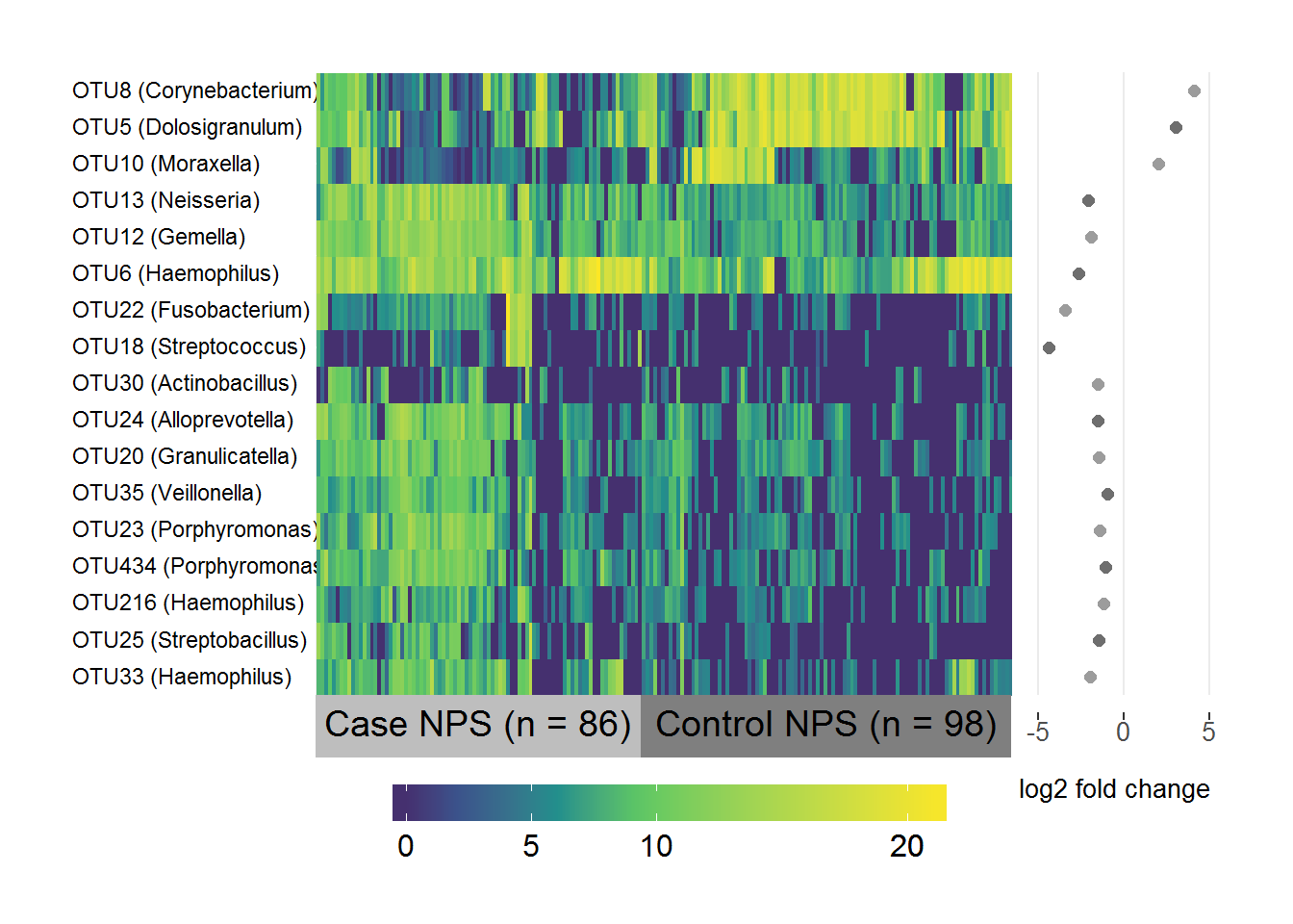

MEF/MER differential abundance

# Subset the normalised logged counts to the OTUs above threshold and in both sets
FR.data <- FR.sig.table[,which(colnames(FR.sig.table) %in% intersect(FR.threshold.1, FR.threshold.2))]

# Transpose it
FR.data <- as.data.frame(t(FR.data))

# Create a list of the fold-change coefficients to be plotted beside the heatmap
FR.coefs <- FR.sig.otus[,1:2]
names(FR.coefs) <- c("OTU", "log2FC")
FR.coefs <- FR.coefs[which(FR.coefs$OTU %in% rownames(FR.data)),]
# Make sure they're in the same order as the data
FR.coefs <- FR.coefs[match(rownames(FR.data), FR.coefs$OTU),]

# Include the genus level taxonomy in the rownames for nice image
FR.taxa <- taxa[,c("taxa", "Genus")]
FR.taxa <- FR.taxa[which(FR.taxa$taxa %in% FR.coefs$OTU),]
# Same order as data
FR.taxa <- FR.taxa[match(FR.coefs$OTU, FR.taxa$taxa), ]
rownames(FR.data) <- paste(rownames(FR.data), " ", "(", FR.taxa$Genus, ")", sep = "")

# Specify the variable to group/label samples by
groupFR <- ifelse(grepl("F", colnames(FR.data)), "Fluids (n = 50)", "Rinses (n = 50)")

# Make heatmap
superheat(FR.data,
          # Sort and label by groupFR (in same order as samples)
          membership.cols = groupFR,
          # Order rows and columns nicely by hierarchical clustering
          pretty.order.rows = TRUE,
          pretty.order.cols = TRUE,
          # Make the OTU labels smaller and align
          left.label.size = 0.35,
          left.label.text.size = 3,
          left.label.text.alignment = "left",
          # Change the colours of the labels
          left.label.col = "White",
          bottom.label.col = c("Grey", "Grey50"),
          # Remove the black lines
          grid.hline = FALSE,
          grid.vline = FALSE,
          # Add the log fold-change plot
          yr = FR.coefs$log2FC,
          yr.axis.name = "log2 fold change")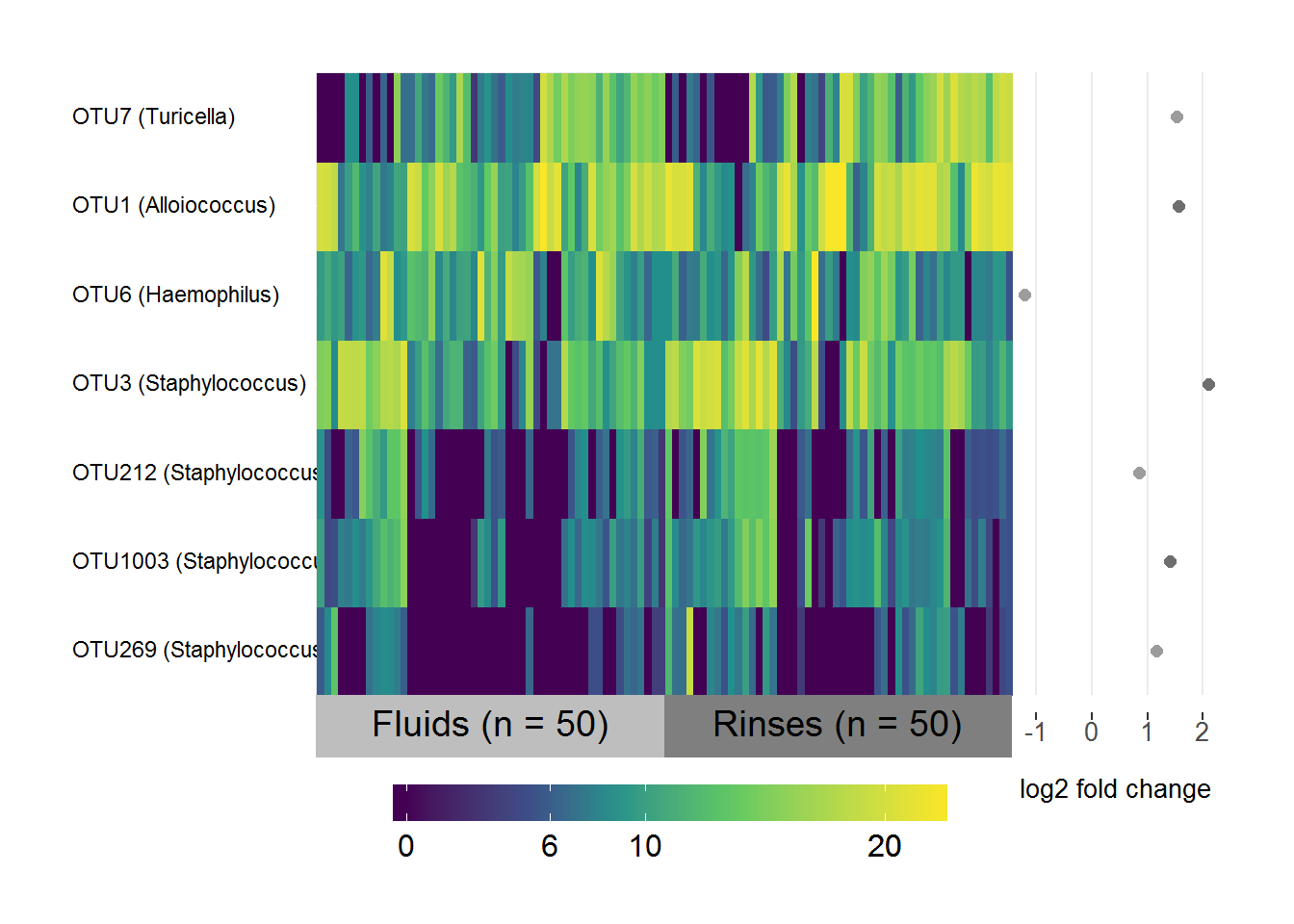

MEF/NPS differential abundance

# Subset the normalised logged counts to the OTUs above threshold and in both sets
FNPS.data <- FNPS.sig.table[,which(colnames(FNPS.sig.table) %in% intersect(FNPS.threshold.1, FNPS.threshold.2))]

# Transpose it
FNPS.data <- as.data.frame(t(FNPS.data))

# Create a list of the fold-change coefficients to be plotted beside the heatmap
FNPS.coefs <- FNPS.sig.otus[,1:2]
names(FNPS.coefs) <- c("OTU", "log2FC")
FNPS.coefs <- FNPS.coefs[which(FNPS.coefs$OTU %in% rownames(FNPS.data)),]
# Make sure they're in the same order as the data
FNPS.coefs <- FNPS.coefs[match(rownames(FNPS.data), FNPS.coefs$OTU),]

# Include the genus level taxonomy in the rownames for nice image
FNPS.taxa <- taxa[,c("taxa", "Genus")]
FNPS.taxa <- FNPS.taxa[which(FNPS.taxa$taxa %in% FNPS.coefs$OTU),]
# Same order as data
FNPS.taxa <- FNPS.taxa[match(FNPS.coefs$OTU, FNPS.taxa$taxa), ]
rownames(FNPS.data) <- paste(rownames(FNPS.data), " ", "(", FNPS.taxa$Genus, ")", sep = "")

# Change Corynebacterium 1 to Corynebacterium for consistency
rownames(FNPS.data) <- gsub("Corynebacterium 1", "Corynebacterium", rownames(FNPS.data))

# Specify the variable to group/label samples by
groupFNPS <- ifelse(grepl("F", colnames(FNPS.data)), "Fluids (n = 75)", "NPS (n = 75)")

# Make heatmap
superheat(FNPS.data,
          # Sort and label by groupFNPS (in same order as samples)
          membership.cols = groupFNPS,
          # Order rows and columns nicely by hierarchical clustering
          pretty.order.rows = TRUE,
          pretty.order.cols = TRUE,
          # Make the OTU labels smaller and align the text
          left.label.size = 0.35,
          left.label.text.size = 3,
          left.label.text.alignment = "left",
          # Change the colours of the labels
          left.label.col = "White",
          bottom.label.col = c("Grey", "Grey50"),
          # Remove the black lines
          grid.hline = FALSE,
          grid.vline = FALSE,
          # Add the log fold-change plot
          yr = FNPS.coefs$log2FC,
          yr.axis.name = "log2 fold change",
          # If you leave default the yr axis only has two ticks)
          yr.lim = c(-6,6))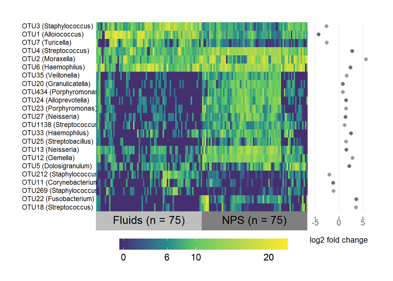

MER/NPS differential abundance

# Subset the normalised logged counts to the OTUs above threshold and in both sets
RNPS.data <- RNPS.sig.table[,which(colnames(RNPS.sig.table) %in% intersect(RNPS.threshold.1, RNPS.threshold.2))]

# Transpose it
RNPS.data <- as.data.frame(t(RNPS.data))

# Create a list of the fold-change coefficients to be plotted beside the heatmap
RNPS.coefs <- RNPS.sig.otus[,1:2]
names(RNPS.coefs) <- c("OTU", "log2FC")
RNPS.coefs <- RNPS.coefs[which(RNPS.coefs$OTU %in% rownames(RNPS.data)),]
# Make sure they're in the same order as the data
RNPS.coefs <- RNPS.coefs[match(rownames(RNPS.data), RNPS.coefs$OTU),]

# Include the genus level taxonomy in the rownames for nice image
RNPS.taxa <- taxa[,c("taxa", "Genus")]
RNPS.taxa <- RNPS.taxa[which(RNPS.taxa$taxa %in% RNPS.coefs$OTU),]
# Same order as data
RNPS.taxa <- RNPS.taxa[match(RNPS.coefs$OTU, RNPS.taxa$taxa), ]
rownames(RNPS.data) <- paste(rownames(RNPS.data), " ", "(", RNPS.taxa$Genus, ")", sep = "")

# Change Corynebacterium 1 to Corynebacterium for consistency
rownames(RNPS.data) <- gsub("Corynebacterium 1", "Corynebacterium", rownames(RNPS.data))

# Specify the variable to group/label samples by
groupRNPS <- ifelse(grepl("S1", colnames(RNPS.data)), "NPS (n = 54)", "Rinses (n = 54)")

# Specify factor levels so you have Rinses on the left and NPS on the right
groupRNPS <- factor(groupRNPS, levels = c("Rinses (n = 54)", "NPS (n = 54)"))

superheat(RNPS.data,
          # Sort and label by groupRNPS (in same order as samples)
          membership.cols = groupRNPS,
          # Order both rows and columns nicely by hierarchical clustering
          pretty.order.rows = TRUE,
          pretty.order.cols = TRUE,
          # Make the OTU labels smaller and align the text
          left.label.size = 0.35,
          left.label.text.size = 3,
          left.label.text.alignment = "left",
          # Change the colours of the labels
          left.label.col = "White",
          bottom.label.col = c("Grey50", "Grey"),
          # Remove the black lines
          grid.hline = FALSE,
          grid.vline = FALSE,
          # Add the log fold-change plot
          yr = RNPS.coefs$log2FC,
          yr.axis.name = "log2 fold change",
          # Nicer scale
          yr.lim = c(-7,7))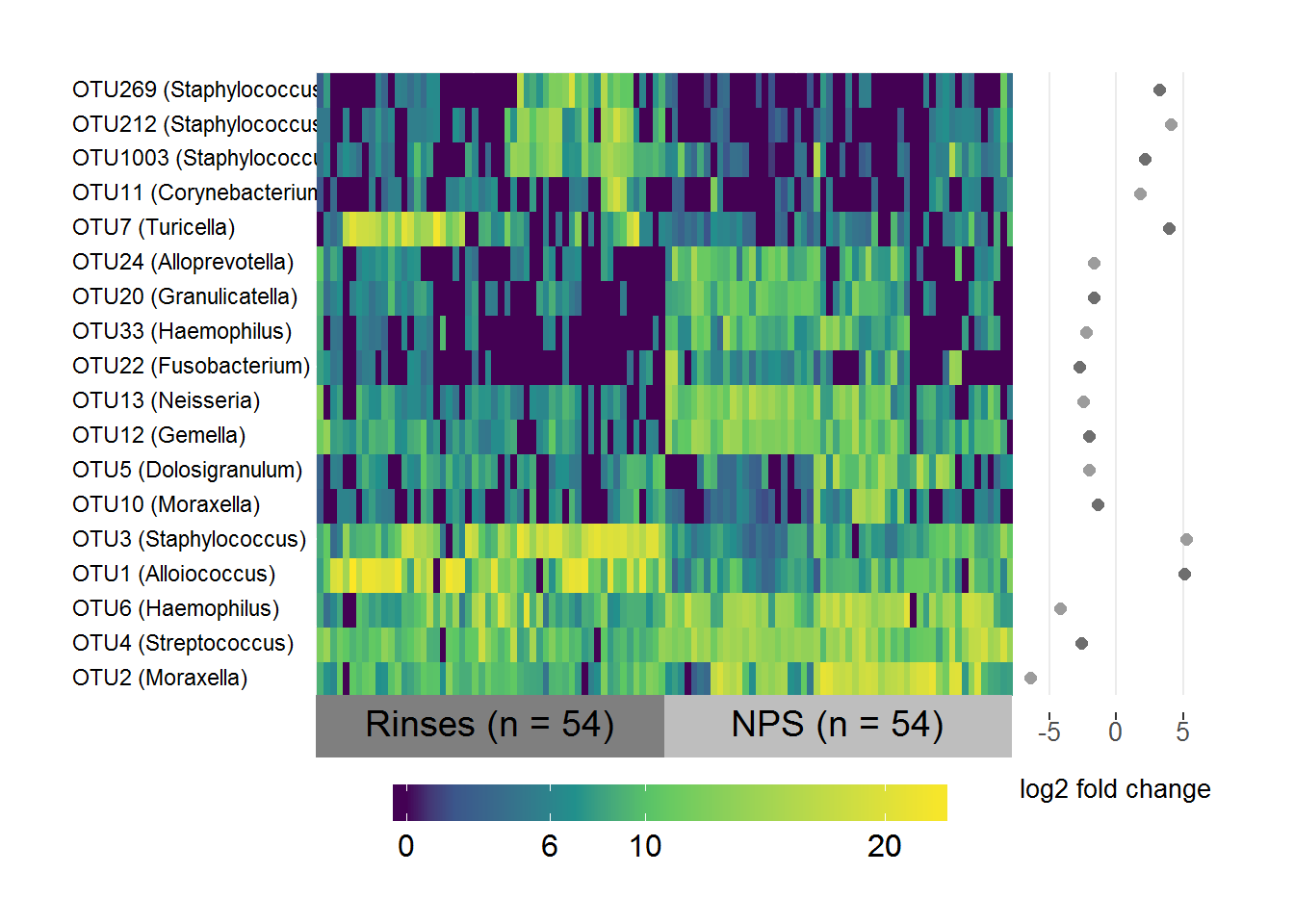

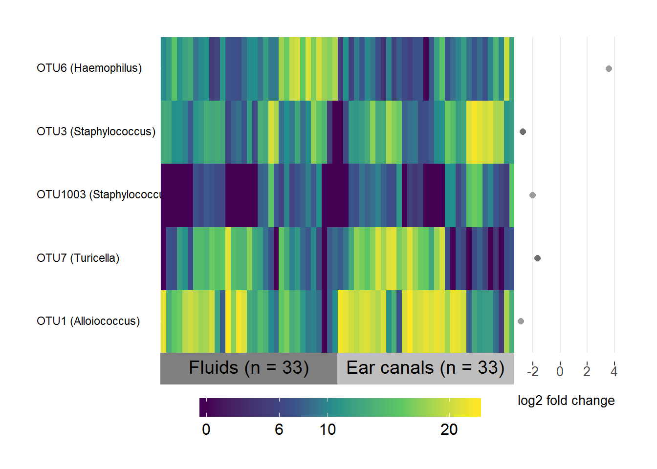
ECS/MEF differential abundance

# Subset the normalised logged counts to the OTUs above threshold
EF.data <- EF.sig.table[,which(colnames(EF.sig.table) %in% EF.threshold)]

# Transpose it
EF.data <- as.data.frame(t(EF.data))

# Create a list of the fold-change coefficients to be plotted beside the heatmap
EF.coefs <- EF.sig.otus[,1:2]
names(EF.coefs) <- c("OTU", "log2FC")
EF.coefs <- EF.coefs[which(EF.coefs$OTU %in% rownames(EF.data)),]
# Make sure they're in the same order as the data
EF.coefs <- EF.coefs[match(rownames(EF.data), EF.coefs$OTU),]

# Include the genus level taxonomy in the rownames for nice image
EF.taxa <- taxa[,c("taxa", "Genus")]
EF.taxa <- EF.taxa[which(EF.taxa$taxa %in% EF.coefs$OTU),]
# Same order as data
EF.taxa <- EF.taxa[match(EF.coefs$OTU, EF.taxa$taxa), ]
rownames(EF.data) <- paste(rownames(EF.data), " ", "(", EF.taxa$Genus, ")", sep = "")

# Specify the variable to group/label samples by
groupEF <- ifelse(grepl("F", colnames(EF.data)), "Fluids (n = 33)", "Ear canals (n = 33)")

# Specify factor levels so you have fluids on the left and canals on the right
groupEF <- factor(groupEF, levels = c("Fluids (n = 33)", "Ear canals (n = 33)"))

superheat(EF.data,
          # Sort and label by groupEF (in same order as samples)
          membership.cols = groupEF,
          # Order the rows and columns nicely by hierarchical clustering
          pretty.order.rows = TRUE,
          pretty.order.cols = TRUE,
          # Make the OTU labels smaller and align the text
          left.label.size = 0.35,
          left.label.text.size = 3,
          left.label.text.alignment = "left",
          # Change the colours of the labels
          left.label.col = "White",
          bottom.label.col = c("Grey", "Grey50"),
          # Remove the black lines
          grid.hline = FALSE,
          grid.vline = FALSE,
           # Add the log fold-change plot
          yr = EF.coefs$log2FC,
          yr.axis.name = "log2 fold change",
          # Nicer scale
          yr.lim = c(-3,4))